Session 29: lme4 Model Criticism & Mixed-Effects Diagnostics

Research Data and Methods Workshop Series — Collaborative Research Centre (CRC 1252) ‘Prominence in Language’

1 Introduction

Linear Mixed-Effects Models (LMMs) and Generalized Linear Mixed-Effects Models (GLMMs) fitted via lme4 (Bates, Mächler, et al. 2015) are widely used in quantitative and experimental linguistics. They can model hierarchically clustered data, handle unbalanced designs, and account for variation across speakers and linguistic materials.

However, standard summary tables can hide assumption violations. A model that converges without error may still violate Gauss-Markov assumptions, have a degenerate random-effects structure (singularity), or be strongly affected by a few participants or unusual stimulus items (Meteyard and Davies 2020).

NoteDatasets

We apply some diagnostic workflows to three linguistic datasets from the ‘languageR’ package (Baayen et al. 2006; Bresnan et al. 2007; Christensen 2019):

1. Continuous Reaction Time LMM (languageR::lexdec) (Baayen et al. 2006): Visual lexical decision reaction times (\(N = 1,659\)) with crossed random factors (21 Subjects crossed with 79 Words), continuous linguistic predictors (Lexical Frequency, Word Length), participant background (NativeLanguage), and experimental progression (Trial).
2. Discrete Syntactic Choice GLMM (languageR::dative) (Bresnan et al. 2007): Dative alternation choices (\(N = 3,263\); double object NP give John the book vs. prepositional PP give the book to John), with predictors related to prominence hierarchies studied in CRC 1252 (Animacy, Pronominality, Givenness, End-Weight).
3. Ordinal Subjective Rating CLMM (languageR::sizeRatings): Semantic size ratings (\(N = 3,078\)) on a 7-point Likert scale across 38 subjects and 81 concrete nouns, used to compare Gaussian and ordinal models.

---

2 Past 10 years

2.1 1. The Random-Effects Complexity Debate (2013)

In an influential paper, Barr et al. (2013) argued that confirmatory hypothesis testing requires “maximal” random-effects structures—including random intercepts and random slopes for all within-unit factors—to avoid Type I error rates rising to 20–40%. However, Bates, Kliegl, et al. (2015) and Matuschek et al. (2017) showed through simulations that maximal models often produce overparameterization, lower statistical power, and singular fits in finite datasets. They recommended data-driven model selection to balance Type I error control and power.

Note: For related simulation-based sample-size and power analyses, see the sequential testing notebook for condition effects, its continuous-predictor counterpart, and the interactive sequential-design sample-size report.

2.2 2. Simulation-Based GLMM Residuals: DHARMa (2016)

Diagnosing Generalized Linear Mixed Models (GLMMs) is difficult because raw, Pearson, and deviance residuals are not easy to interpret for discrete binary and count outcomes. Florian Hartig (2022) introduced simulation-based quantile residuals using the Probability Integral Transform (PIT). DHARMa uses these residuals to test uniformity, overdispersion, and zero-inflation.

2.3 3. Ben Bolker’s Convergence Tooling & glmmTMB (continuously updated)

As lead maintainer of lme4, Ben Bolker helped develop tools for investigating optimization warnings (Bolker et al. 2009). Relevant tools include:

• lme4::allFit(): Benchmarking models across multiple derivative-free optimizers to detect false-positive convergence warnings.
• lme4::isSingular(): Mathematical boundary checking based on Cholesky factor singular values.
• glmmTMB (Brooks et al. 2017): Flexible template-model-builder architecture handling complex dispersion, zero-inflation, and spatial/temporal autocorrelation structures.
• trouBBlme4SolveR: Automated diagnostic routines to resolve boundary singularities.

2.4 4. Model Checks with easystats (2020)

The easystats packages (Lüdecke et al. 2021) provide tools for model diagnostics and summaries:

• performance::check_model(): A visual overview covering linearity, homoscedasticity, posterior predictive checks, collinearity, and random-effect normality.
• performance::r2_nakagawa(): Estimates marginal and conditional \(R^2\) (Nakagawa and Schielzeth 2013).

For Bayesian alternatives, see the brms posterior predictive checks notebook.

2.5 5. Marginal Effects (2016)

Russell Lenth’s emmeans (2016) and Vincent Arel-Bundock’s marginaleffects (2024) provide tools for post-hoc contrasts, reference grids, and response-scale predictions.

2.6 6. Bayesian Models with brms (2017)

Paul-Christian Bürkner’s brms (2017) provides an interface to Hamiltonian Monte Carlo (HMC) estimation through Stan. As Vasishth et al. (2018) discuss, weakly informative priors (see Setting Priors in brms) can regularize boundary estimates while retaining scientifically motivated random slopes.

---

3 Assumptions

The table below compares assumptions in classical ANOVA and Bayesian mixed models:

Assumption Dimension	RM-ANOVA	lme4 Linear (LMM)	lme4 Generalized (GLMM)	Bayesian Mixed Models (brms)	Modern Diagnostic Tool
Design Balance	Strict balance required; listwise deletion for missing cells	Unbalanced cells and missing observations handled natively	Unbalanced cells and missing observations handled natively	Unbalanced cells and missing observations handled natively	Missingness summaries (summary(), colSums(is.na(data)))
Sphericity	Required; violated sphericity inflates \(F\)-test Type I errors	Relaxed: Variance-covariance components modeled directly	Relaxed: Variance-covariance components modeled directly	Relaxed: Full covariance prior (e.g. LKJ) modeled directly	Mauchly’s test and Greenhouse-Geisser/Huynh-Feldt corrections (ANOVA only)
Crossed Item Variation	Violated: Language-as-fixed-effect problem (Clark 1973)	Satisfied: Crossed random intercepts & slopes (Subject + Word)	Satisfied: Crossed random structures	Satisfied: Crossed random structures with regularizing priors	Crossed formula syntax: (1 | Subject) + (1 | Word)
Residual Distribution	\(\epsilon \sim \mathcal{N}(0, \sigma^2)\)	\(\epsilon \sim \mathcal{N}(0, \sigma^2)\) (Normality required)	Uniform quantile residuals \(\mathcal{U}(0,1)\) via PIT	Full posterior predictive distribution matching data family	Q-Q plots, performance::check_model(), DHARMa::testUniformity()
Homoscedasticity (‘scatterness’ of variance)	Equal variance across groups required	Homoscedastic residual variance \(\sigma^2\) assumed	Variance coupled to mean (\(\mu(1-\mu)\)); overdispersion can invalidate the model	Can model residual variance as distributional regression (sigma ~ ...)	Residual-vs-fitted/scale-location plots, performance::check_heteroscedasticity(), DHARMa::testDispersion()
Linearity & Scaling	Linear relationships assumed	Linear on response scale; scale continuous predictors	Linear on link scale (log, logit, probit, cloglog)	Linear or non-linear on link scale	Partial residual plots and performance::check_model()
Multicollinearity (predictor collinearity)	Correlated predictors make effects non-orthogonal and less precise	Correlated fixed predictors inflate standard errors and destabilize estimates	Collinearity can destabilize estimates, especially with sparse outcomes	Priors can regularize estimates but cannot replace information absent from data	performance::check_collinearity(), predictor correlation matrix (cor())
Random Effects Normality	N/A	BLUPs assumed multivariate normal: \(b \sim \mathcal{N}(0, \Sigma)\)	Conditional modes assumed multivariate normal	Priors specify random-effects distributions (Normal, Student-\(t\))	Q-Q plots of BLUPs, performance::check_model()
Singularity & Boundaries	N/A	Boundary estimates (\(\sigma_b^2 = 0, \rho = \pm 1\)) can occur	Laplace approximation may have difficulty near boundaries	Regularizing priors can reduce boundary estimates	lme4::isSingular(), lme4::rePCA(), lme4::allFit()
Residual Independence	Assumed across trials	Assumed; sequential trial fatigue violates independence	Assumed; temporal/spatial clustering violates independence	Autoregressive structures can be added (ar(), cor_ar())	acf(), performance::check_autocorrelation(), DHARMa::testTemporalAutocorrelation()

---

4 Environment Setup

# Core mixed-effects modeling
library(lme4)
library(lmerTest)

# Simulation-based residual diagnostics
library(DHARMa)

# Multi-panel model checks & Nakagawa R-squared
library(performance)
library(parameters)
library(see)

# Cluster-level influence diagnostics
library(influence.ME)

# Automated singularity & convergence troubleshooting
library(trouBBlme4SolveR)
library(dfoptim)

# Publication tables
library(knitr)

# Ordinal mixed models
library(ordinal)

# Post-hoc contrasts and estimated marginal means
library(emmeans)

# Linguistic benchmark datasets
library(languageR)

# Tidyverse data wrangling and plotting
library(tidyverse)

# Reproducibility seed & visualization theme
set.seed(12345)
theme_set(theme_minimal(base_size = 12))

---

5 Module 1: LMMs, Reaction Times & Singularity

5.1 1.1 Random Effects Syntax

5.1.1 Overview:

Mixed-effects models relax the rigid balanced-design and sphericity assumptions of repeated-measures ANOVA:

• Nested random effects (e.g., Students nested within Classrooms): (1 | Class / Student) expands to (1 | Class) + (1 | Class:Student).
• Crossed random effects (e.g., Participants crossed with Stimulus Words): (1 | Subject) + (1 | Word)
• Interaction operator :: (1 | Subject:Word) gives a random intercept for each observed Subject-Word pairing; use it when pair-specific variation is part of the design.
• Correlated random intercept and slope: (1 + x | Subject) estimates their correlation as well as their variances.
• Slope without an intercept: (0 + x | Subject) estimates a subject-specific slope for x without a subject-specific intercept; 0 + removes the intercept term.
• Uncorrelated random intercept and slope: For numeric x, (1 + x || Subject) expands to (1 | Subject) + (0 + x | Subject), fitting the terms without their correlation. Compare (1 + x | Subject) (3 parameters) with (1 + x || Subject) (2 parameters). Fewer parameters make a singular fit less likely, but the model then assumes, for example, that subjects with slow baselines are no more or less sensitive to x than others.
• diag(): the name of the same idea in glmmTMB, where a covariance structure is written as a function around the term: diag(1 + x | Subject) means a diagonal covariance matrix (variances only, zero correlations). Other choices there include us() (unstructured, the default |), cs() (compound symmetry), and ar1() (autoregressive). Plain lme4 has no diag(); there the double bar is the only shorthand for this structure.

WarningNote

|| only removes the correlations reliably for numeric predictors. If x is a factor with more than two levels, lme4 splits the term before it creates the dummy (contrast) columns, so the columns of the factor can stay correlated with each other. For factors, first create numeric contrast columns (as done below with Native_num and Sex_num) and use those inside ||, or write out the separate (0 + ... | ...) terms.

We prepare languageR::lexdec (Baayen et al. 2006), standardizing continuous predictors to optimize numerical conditioning and applying centered sum contrast coding (\(-0.5 / +0.5\)) to categorical factors (Schad et al. 2020):

# Load lexical decision dataset from languageR (Baayen et al., 2006)
data(lexdec)

# 1. Rescale continuous predictors to z-scores (mean = 0, sd = 1)
#    This eliminates scale disparities and avoids ill-conditioned deviance valleys
# 2. Apply centered sum contrast coding (-0.5 / +0.5) to two-level factors
#    Ensures intercept represents grand mean and beta represents true main effects
lexdec <- lexdec %>%
  mutate(
    Freq_z     = as.numeric(scale(Frequency)),
    Length_z   = as.numeric(scale(Length)),
    Native_num = ifelse(NativeLanguage == "Other", 0.5, -0.5),
    Sex_num    = ifelse(Sex == "M", 0.5, -0.5)
  )

# Inspect processed variables
glimpse(select(lexdec, Subject, Word, RT, Trial, Freq_z, Length_z, Native_num, Sex_num))

Rows: 1,659
Columns: 8
$ Subject    <fct> A1, A1, A1, A1, A1, A1, A1, A1, A1, A1, A1, A1, A1, A1, A1,…
$ Word       <fct> owl, mole, cherry, pear, dog, blackberry, strawberry, squir…
$ RT         <dbl> 6.340359, 6.308098, 6.349139, 6.186209, 6.025866, 6.180017,…
$ Trial      <int> 23, 27, 29, 30, 32, 33, 34, 38, 41, 42, 45, 46, 47, 48, 53,…
$ Freq_z     <dbl> 0.085255426, -0.114461645, 0.193018975, -0.018605419, 2.287…
$ Length_z   <dbl> -1.56745815, -1.02907035, 0.04770525, -1.02907035, -1.56745…
$ Native_num <dbl> -0.5, -0.5, -0.5, -0.5, -0.5, -0.5, -0.5, -0.5, -0.5, -0.5,…
$ Sex_num    <dbl> -0.5, -0.5, -0.5, -0.5, -0.5, -0.5, -0.5, -0.5, -0.5, -0.5,…

ImportantContrast Coding

In R, factors default to treatment (dummy) coding (contr.treatment), which maps the first alphabetical level to 0 and all other levels to 1. With interactions and random slopes, this coding affects how model coefficients are interpreted and can affect the fitted random-effects correlations (Schad et al. 2020):

1. Misinterpretation of Main Effects: In models with interactions (\(A \times B\)), the lower-order \(\beta\) coefficients under treatment coding are not main effects; they are simple effects restricted specifically to the arbitrary baseline level of the other factor.
2. Random Slope Correlations: In (1 + Condition | Subject), treatment coding defines the random intercept at the baseline condition. Depending on the data, this can increase dependence between intercept and slope estimates and contribute to correlations near \(\pm 1.0\) or singular fits.
3. Type III ANOVA Tables: Type III tests (car::Anova(type = "III")) are often used with sum contrasts (contr.sum). With treatment coding, the tests may not answer the intended question.

Centered sum coding (\(-0.5 / +0.5\)) centers the intercept at the unweighted grand mean across conditions, decouples random intercepts from random slopes, and ensures \(\beta\) coefficients represent true main effects.

5.2 1.2 A Maximal Model (Barr et al., 2013)

According to Barr et al. (2013), any factor varying within a grouping unit must have a corresponding random slope.

# Fit maximal random-effects model (Barr et al., 2013)
# Random intercepts and within-unit random slopes for all predictors:
# - Within Subject: Frequency and Word Length
# - Within Word: Native Language and Speaker Sex
m_maximal <- lmer(
  RT ~ Freq_z + Length_z + Native_num + Sex_num +
    (1 + Freq_z + Length_z | Subject) +
    (1 + Native_num + Sex_num | Word),
  data = lexdec
)

# Test for singularity (Cholesky factor on boundary)
cat("Is the maximal model singular?", isSingular(m_maximal), "\n")

Is the maximal model singular? TRUE 

5.3 1.3 Singularity

When isSingular() returns TRUE, the variance-covariance matrix lies on the boundary:

# Inspect estimated variance-covariance matrices and correlation parameters (rho)
# Look for variances collapsing to 0.000 or correlations at +/- 1.000
print(VarCorr(m_maximal))

 Groups   Name        Std.Dev. Corr          
 Word     (Intercept) 0.052695               
          Native_num  0.034887  0.760        
          Sex_num     0.017057 -0.799 -0.998 
 Subject  (Intercept) 0.142156               
          Freq_z      0.018882 -0.433        
          Length_z    0.023391  0.920 -0.473 
 Residual             0.168189               

rePCA() gives a complementary view by rotating each grouping factor’s random-effects covariance into orthogonal principal components. Near-zero component standard deviations reveal unsupported directions, including combinations of intercepts and slopes that may not be obvious in VarCorr().

# Inspect standard deviations of orthogonal random-effects components
print(rePCA(m_maximal))

$Word
Standard deviations (1, .., p=3):
[1] 0.3682386 0.1259937 0.0000000

Rotation (n x k) = (3 x 3):
           [,1]       [,2]       [,3]
[1,] -0.8291107  0.5583410 0.02882327
[2,] -0.4992204 -0.7625591 0.41143965
[3,]  0.2517031  0.3267398 0.91098114

$Subject
Standard deviations (1, .., p=3):
[1] 0.85630446 0.10177525 0.05214466

Rotation (n x k) = (3 x 3):
            [,1]        [,2]       [,3]
[1,] -0.98696881 -0.07898606 -0.1401919
[2,]  0.05780677 -0.98711757  0.1491887
[3,] -0.15016969  0.13914057  0.9788202

attr(,"class")
[1] "prcomplist"

WarningSingular Fit in the Maximal Model

The Word random-intercept standard deviation is 0.000, with a boundary correlation of 1.000. This fit does not support estimating separate item-level slopes for speaker background factors alongside the intercepts (Bates, Kliegl, et al. 2015).

5.4 1.4 Automated Singularity Resolution (trouBBlme4SolveR)

The trouBBlme4SolveR::dwmw() function identifies zero-variance random slopes and removes them iteratively:

# Automated troubleshooting for singular fits (Ben Bolker's trouBBlme4SolveR)
# 'dwmw' ("Don't Worry, Make Warmer") iteratively tests and prunes zero-variance random slopes
m_resolved <- dwmw(m_maximal)
cat("\nIs resolved model singular?", isSingular(m_resolved), "\n")

Is resolved model singular? FALSE 

print(summary(m_resolved))

Linear mixed model fit by REML. t-tests use Satterthwaite's method [
lmerModLmerTest]
Formula: RT ~ Freq_z + Length_z + Native_num + Sex_num + (1 + Freq_z +  
    Length_z | Subject) + (1 + Native_num | Word)
   Data: lexdec

REML criterion at convergence: -976.9

Scaled residuals: 
    Min      1Q  Median      3Q     Max 
-2.2258 -0.6208 -0.1123  0.4417  6.3908 

Random effects:
 Groups   Name        Variance  Std.Dev. Corr        
 Word     (Intercept) 0.0030403 0.05514              
          Native_num  0.0012923 0.03595  0.83        
 Subject  (Intercept) 0.0201153 0.14183              
          Freq_z      0.0003597 0.01897  -0.43       
          Length_z    0.0005399 0.02324   0.92 -0.46 
 Residual             0.0283971 0.16851              
Number of obs: 1659, groups:  Word, 79; Subject, 21

Fixed effects:
             Estimate Std. Error        df t value Pr(>|t|)    
(Intercept)  6.392940   0.033065 19.613673 193.345  < 2e-16 ***
Freq_z      -0.044294   0.008835 44.949596  -5.013 8.82e-06 ***
Length_z     0.016890   0.009332 44.562639   1.810   0.0771 .  
Native_num   0.071470   0.045791 20.031541   1.561   0.1342    
Sex_num      0.016473   0.046209 18.000358   0.356   0.7256    
---
Signif. codes:  0 '***' 0.001 '**' 0.01 '*' 0.05 '.' 0.1 ' ' 1

Correlation of Fixed Effects:
           (Intr) Freq_z Lngth_ Ntv_nm
Freq_z     -0.187                     
Length_z    0.456  0.188              
Native_num  0.158  0.009 -0.127       
Sex_num     0.252  0.000  0.000  0.196

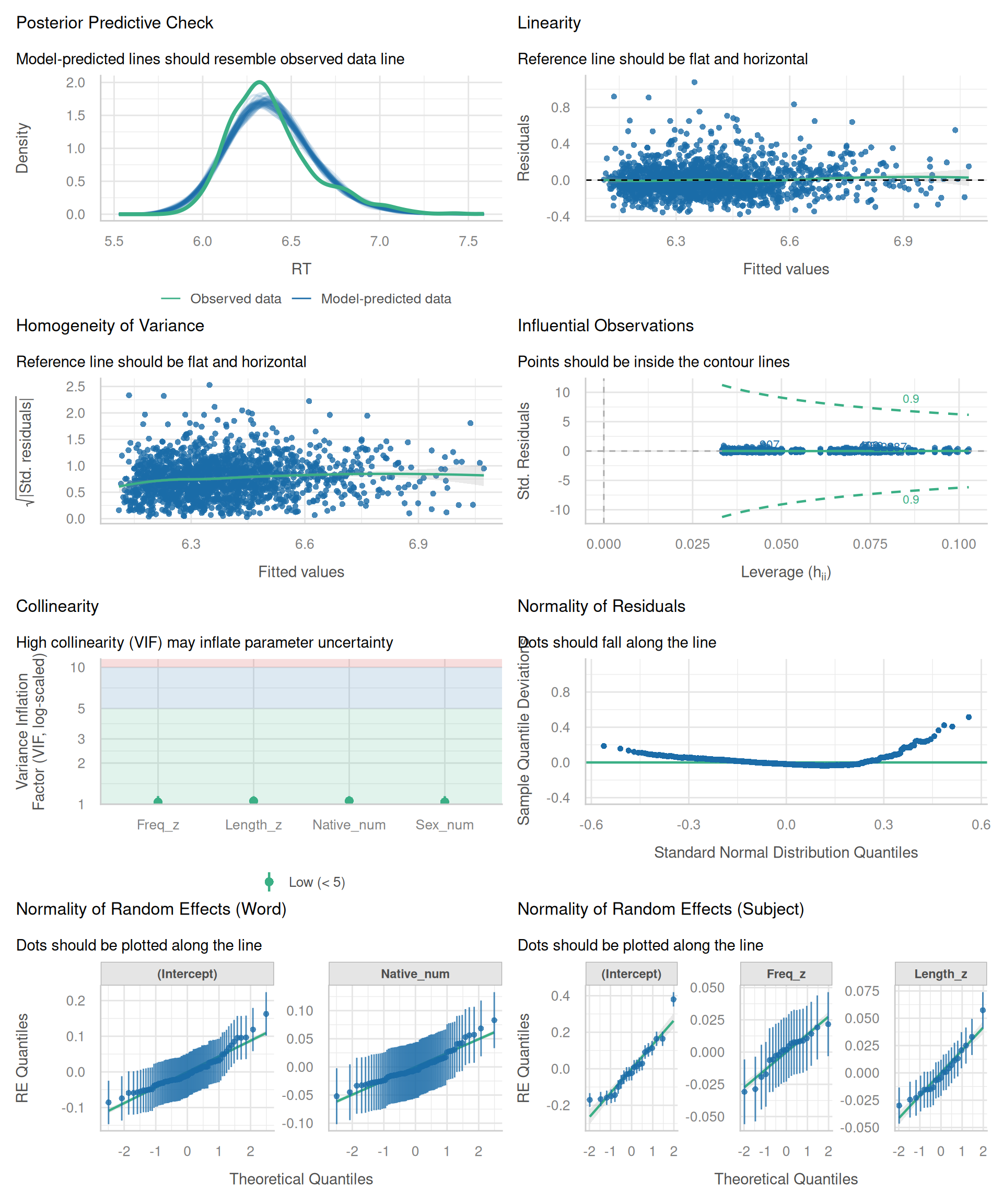
performance::check_model() gives a visual overview of the resolved model: linearity, homogeneity of variance, posterior predictive fit, influential observations, collinearity, and normality of the residuals and of the random effects.

check_model(m_resolved)

How to read each panel

• Posterior predictive check: The blue lines are data simulated from the model, and the green line is the observed RT distribution. They agree on location and spread, and the tails match. The observed peak is slightly higher and narrower than the simulated ones, so the model spreads a little too much probability away from the mode. This is a minor mismatch.
• Linearity: The reference line should be flat at zero. It is, so there is no sign of curvature between fitted values and residuals. A few large positive residuals (up to about 1 log unit) are the slow responses that also show up in the residual Q-Q panel.
• Homogeneity of variance: The reference line should be flat. It rises only slightly, and the spread of the points is similar across fitted values. There is no strong heteroscedasticity.
• Influential observations: Points outside the dashed contour lines would be both high-leverage and poorly fitted. None fall outside, so no single trial dominates the fit. Note that the standardized residuals here are compressed near zero, so this panel is less informative for mixed models than the cluster-level checks in Module 3.
• Collinearity: All variance inflation factors are close to 1, well below the rule-of-thumb threshold of 5, so the predictors do not overlap enough to destabilize the estimates.
• Normality of residuals: This is a detrended Q-Q plot, so a perfect fit would lie on the horizontal line. The middle follows it, but the upper tail lifts away, up to about 0.5. This is the same heavy right tail (a few very slow responses) discussed in Module 2. It is a real but modest departure, and Module 2 checks whether it affects the results.
• Normality of random effects (Word and Subject): The dots should follow the line, given their intervals. The intercepts and slopes for both Word and Subject stay close to it, with small deviations only at the extremes where intervals are wide. There is no clear evidence against normally distributed random effects.

Conclusion: The model shows no major violations. The main concern is the heavy upper tail of the residuals, which is small enough that it should be checked with a sensitivity analysis rather than treated as a reason to reject the model.

---

6 Module 2: GLMMs, Dative Alternation & DHARMa

6.1 2.1 Classical Residual Checks in Linear Mixed Models

In standard Gaussian LMMs, residuals are assumed to follow \(\epsilon \sim \mathcal{N}(0, \sigma^2)\):

# Parsimonious random-effects model (Bates et al., 2015)
# Retains subject-level frequency slope; prunes overparameterized item slopes
m_parsimonious <- lmer(
  RT ~ Freq_z + Length_z + Native_num + (1 + Freq_z | Subject) + (1 | Word),
  data = lexdec
)

# Classical diagnostic plots for Gaussian LMM:
# Left: Normal Q-Q plot to assess residual normality (epsilon ~ N(0, sigma^2))
# Right: Residuals vs. Fitted to assess homoscedasticity and linearity
par(mfrow = c(1, 2))
qqnorm(residuals(m_parsimonious), main = "Normal Q-Q Plot (Raw Residuals)")
qqline(residuals(m_parsimonious), col = "red", lwd = 2)

plot(fitted(m_parsimonious), residuals(m_parsimonious),
     xlab = "Fitted Values (log RT)", ylab = "Residuals",
     main = "Residuals vs. Fitted", pch = 16, col = rgb(0,0,0,0.2))
abline(h = 0, col = "red", lty = 2, lwd = 2)

par(mfrow = c(1, 1))

How to read these plots

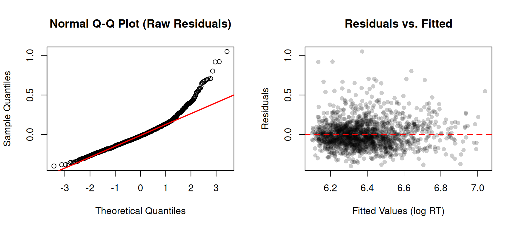
• Q-Q plot (left): If the residuals are normal, the points lie on the red line. Here the middle of the distribution follows the line closely, but the upper tail bends clearly away from it. A group of responses are much slower than a normal distribution predicts (a right-skewed, heavy upper tail). This is common in reaction-time data, even after a log transformation. The lower tail deviates only slightly.
• Residuals vs. fitted (right): You want an even, structureless band around the dashed zero line. There is no obvious curve, so linearity looks adequate, and the spread is roughly constant across fitted values. The few large positive residuals are the same slow responses seen in the Q-Q plot.

Conclusion: The mean structure and variance look reasonable, but the heavy upper tail is a real departure from normality. With 1,659 observations, fixed-effect estimates are often fairly robust to this kind of non-normality, but standard errors and p-values can be affected, so check it with the simple follow-ups below.

Simple follow-up checks

1. Count how many residuals are extreme (more than 2.5 standard deviations from zero).
2. Check whether they cluster in particular participants or words. If they do, look at those clusters (see the influence diagnostics in Module 3).
3. Refit without the extreme observations and compare the fixed effects. If estimates and conclusions barely change, the tail is not driving your results. If they change, report both models and consider a different transformation or response distribution.

# Standardized residuals: |z| > 2.5 flags unusually slow or fast trials
res_std <- as.numeric(scale(residuals(m_parsimonious)))
extreme <- abs(res_std) > 2.5

# 1. How many extreme residuals?
cat("Extreme residuals:", sum(extreme), "of", length(res_std), "\n")

Extreme residuals: 36 of 1659 

# 2. Do they cluster in particular subjects or words?
head(sort(table(lexdec$Subject[extreme]), decreasing = TRUE), 5)

A1  I M2 R3 A2 
 4  3  3  3  2 

head(sort(table(lexdec$Word[extreme]), decreasing = TRUE), 5)

crocodile  hedgehog      leek    almond       ant 
        2         2         2         1         1 

# 3. Sensitivity refit without them: do the fixed effects change?
m_trimmed <- update(m_parsimonious, data = lexdec[!extreme, ])
round(cbind(full = fixef(m_parsimonious), trimmed = fixef(m_trimmed)), 3)

              full trimmed
(Intercept)  6.390   6.377
Freq_z      -0.047  -0.044
Length_z     0.017   0.016
Native_num   0.071   0.080

Interpret the last table by comparing the two columns. Similar estimates with the same sign and size mean the conclusions do not depend on the extreme trials.

In this dataset, 36 of 1,659 trials (about 2%) are extreme. They are spread over many subjects and words rather than concentrated in a few, and the fixed effects barely change after removing them (for example, Freq_z moves from -0.047 to -0.044). The heavy tail is therefore visible in the plot but does not drive the conclusions.

6.2 2.2 Discrete GLMM Residuals

6.2.1 Why standard residual plots fail for discrete outcomes

In a Gaussian LMM, a residual is \(y_i - \hat{y}_i\). If the model is correct, these residuals have the same roughly normal shape at every fitted value, so a normal Q-Q plot and a residuals-vs-fitted plot can reveal problems.

In a logistic GLMM this breaks down, even when the model is correct:

• The residuals can take only two values per fitted value. Suppose the model predicts \(\hat{p}_i = 0.8\). The observed outcome is either 0 or 1, so the raw residual is either \(-0.8\) or \(+0.2\), never anything in between. Plotted against the fitted values, the residuals fall on two diagonal bands (\(-\hat{p}\) and \(1 - \hat{p}\)) instead of forming a cloud.
• Rescaling does not fix this. Pearson residuals, \((y_i - \hat{p}_i) / \sqrt{\hat{p}_i(1 - \hat{p}_i)}\), and deviance residuals are still a function of one of two outcomes at each \(\hat{p}_i\), so they form curved bands and are far from normal.
• The variance depends on the mean. For a binary outcome, \(\text{Var}(y_i) = \hat{p}_i(1 - \hat{p}_i)\). Unequal spread across fitted values is therefore expected and is not evidence of heteroscedasticity in the sense used for LMMs.
• The reference distribution is unclear. There is no simple “should look like this” pattern, so a Q-Q plot against the normal distribution or a smoother through the residuals cannot separate real misfit from these built-in artifacts. The same applies to counts with few distinct values, such as low-rate Poisson data.

The practical consequence is that a bad-looking standard residual plot does not show that the model is wrong, and a good-looking one does not show that it is right.

6.2.2 What DHARMa does instead

The DHARMa package (Hartig 2022) turns residuals of any model family into a common, interpretable scale, using simulation:

1. Simulate many new datasets (for example, 250 or 500) from the fitted model, including its random effects.
2. For each observation, find where the observed value falls within the distribution of the simulated values for that same observation. This gives a scaled residual between 0 and 1, computed with the Probability Integral Transform (PIT): \[u_i = P(Y^{\text{sim}}_i \le y_i) \sim \mathcal{U}(0, 1)\]
3. For discrete outcomes, many simulated values tie, so DHARMa randomizes the position within the tie. This is what makes the residuals continuous.

If the model is correctly specified, the scaled residuals are uniformly distributed between 0 and 1, whatever the family (binomial, Poisson, Gaussian). A residual of 0.5 means the observation was at the median of what the model predicts, and values near 0 or 1 mean it was unusually low or high.

This gives one uniform reference for every model type:

• A uniform Q-Q plot checks whether the overall distribution is compatible with the model.
• Residuals vs. predicted values should show no trend and roughly flat quantile lines.
• Formal tests (testUniformity(), testDispersion(), testZeroInflation()) check specific problems, such as over- or underdispersion or excess zeros, against the simulated expectation.

DHARMa does not remove the need for judgment. With many observations, the tests can flag small deviations that do not matter, so compare the plots with the test results.

6.3 2.3 Data: Dative Alternation

We model the English dative alternation (Bresnan et al. 2007), where prominence features (animate recipients, pronominal recipients, short themes) predict the double-object construction (NP) versus prepositional construction (PP):

# Discrete Prominence GLMM: English Dative Alternation (Bresnan et al., 2007)
# Binary outcome: Realization of recipient as NP (double object) vs PP (prepositional)
data(dative)

m_dative <- glmer(
  RealizationOfRecipient ~ AnimacyOfRec + PronomOfRec + LengthOfTheme + (1 | Verb),
  family = binomial,
  data = dative
)
summary(m_dative)

Generalized linear mixed model fit by maximum likelihood (Laplace
  Approximation) [glmerMod]
 Family: binomial  ( logit )
Formula: RealizationOfRecipient ~ AnimacyOfRec + PronomOfRec + LengthOfTheme +  
    (1 | Verb)
   Data: dative

      AIC       BIC    logLik -2*log(L)  df.resid 
   2245.6    2276.0   -1117.8    2235.6      3258 

Scaled residuals: 
    Min      1Q  Median      3Q     Max 
-3.6492 -0.3311 -0.1865  0.1243 23.9501 

Random effects:
 Groups Name        Variance Std.Dev.
 Verb   (Intercept) 3.272    1.809   
Number of obs: 3263, groups:  Verb, 75

Fixed effects:
                      Estimate Std. Error z value Pr(>|z|)    
(Intercept)            1.42924    0.29130   4.906 9.28e-07 ***
AnimacyOfRecinanimate  1.14478    0.18633   6.144 8.06e-10 ***
PronomOfRecpronominal -2.46711    0.12257 -20.128  < 2e-16 ***
LengthOfTheme         -0.28716    0.02266 -12.671  < 2e-16 ***
---
Signif. codes:  0 '***' 0.001 '**' 0.01 '*' 0.05 '.' 0.1 ' ' 1

Correlation of Fixed Effects:
            (Intr) AnmcOR PrnmOR
AnmcyOfRcnn -0.036              
PrnmOfRcprn -0.228 -0.015       
LengthOfThm -0.305  0.004  0.279

# DHARMa: Simulate standardized quantile residuals via Probability Integral Transform (PIT)
# Residuals are transformed to Uniform U(0, 1) under the null of correct specification
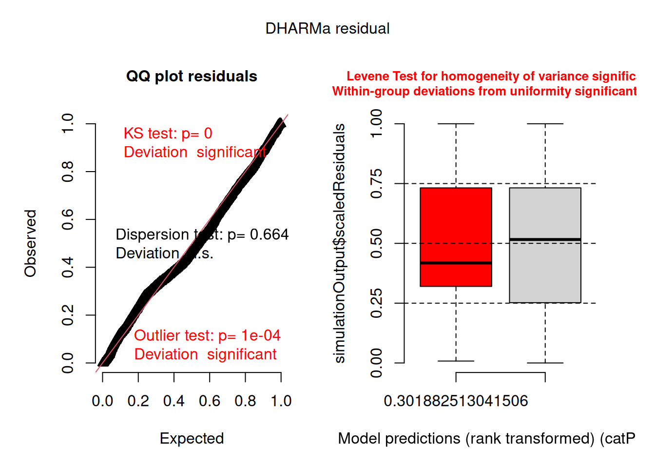
sim_dative <- simulateResiduals(fittedModel = m_dative, n = 500, plot = FALSE)

# DHARMa 2-panel diagnostic plot: Uniform Q-Q plot and Residuals vs. Predicted with spline
plot(sim_dative)

How to read the DHARMa plot

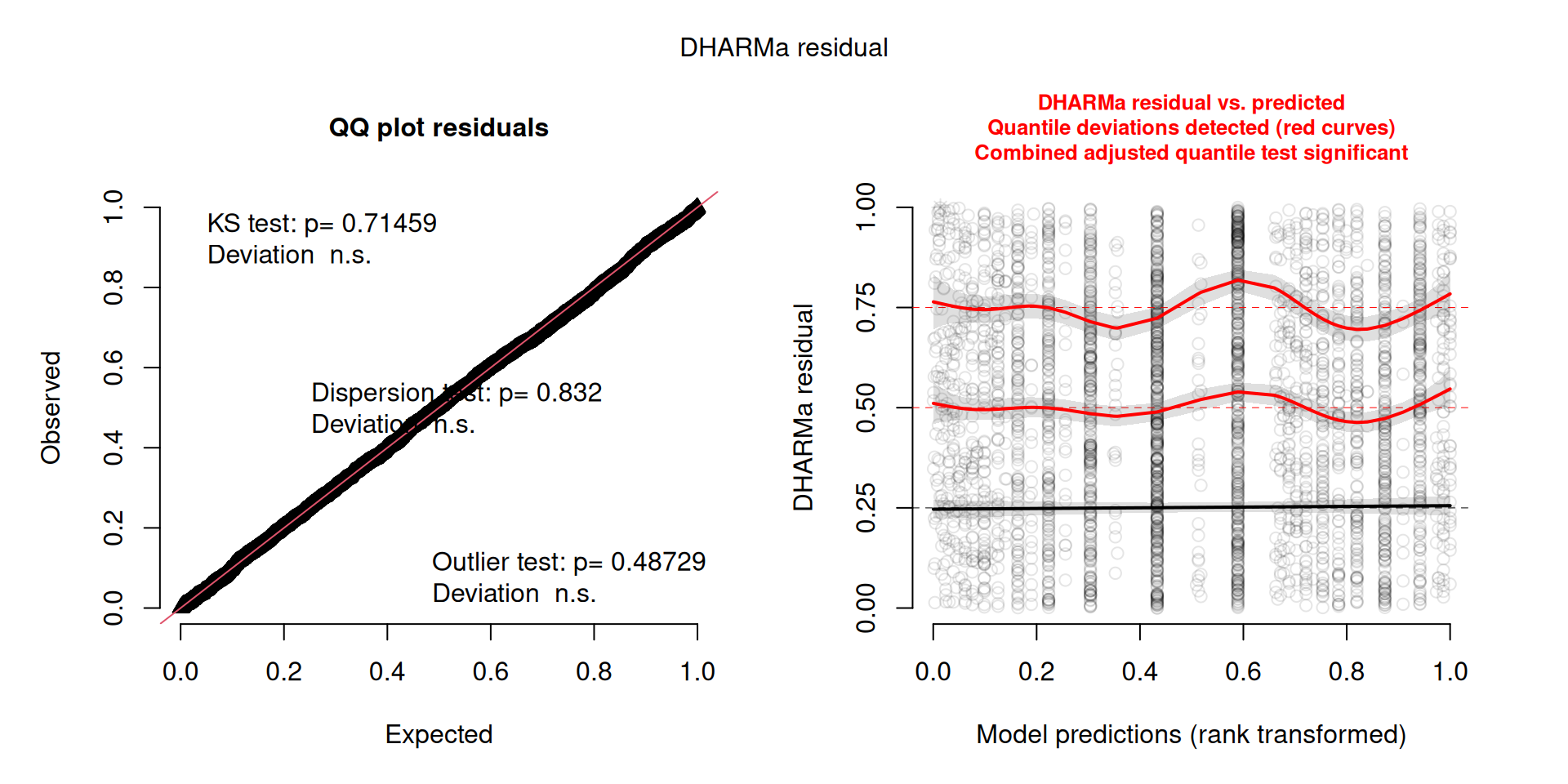
• QQ plot residuals (left): Under a correct model, the scaled residuals are uniform, so the points lie on the diagonal. They do, and the three tests printed on the plot are all non-significant: uniformity (KS test, \(p = 0.71\)), dispersion (\(p = 0.83\)), and outliers (\(p = 0.49\)). The overall distribution of the residuals is compatible with the model.
• DHARMa residual vs. predicted (right): The three solid curves are smoothed quantiles (25%, 50%, 75%) of the residuals across the model’s predictions, and the dashed lines show where they should be if the model is correct. The curves wobble around the dashed lines (the 75% curve rises to about 0.82 near the middle of the range and dips to about 0.70 elsewhere), and DHARMa reports “quantile deviations detected” in red. The vertical stripes are not a problem: the predictors are mostly categorical, so many observations share the same prediction.

Conclusion: The model reproduces the overall distribution of the outcome, but the predicted probabilities are not calibrated equally well across the range. With 3,263 observations the quantile test is sensitive, and the deviations are moderate, so treat this as a sign of possible misspecification rather than a failure. Possible causes are a missing predictor, a non-linear effect (for example, of LengthOfTheme), or a missing interaction. Plotting the residuals against each predictor with plotResiduals() shows where the pattern comes from.

# Scaled residuals against each predictor: flat quantile lines mean no unmodelled pattern
par(mfrow = c(1, 3))
plotResiduals(sim_dative, dative$AnimacyOfRec, xlab = "AnimacyOfRec")
plotResiduals(sim_dative, dative$PronomOfRec, xlab = "PronomOfRec")
plotResiduals(sim_dative, dative$LengthOfTheme, xlab = "LengthOfTheme")

par(mfrow = c(1, 1))

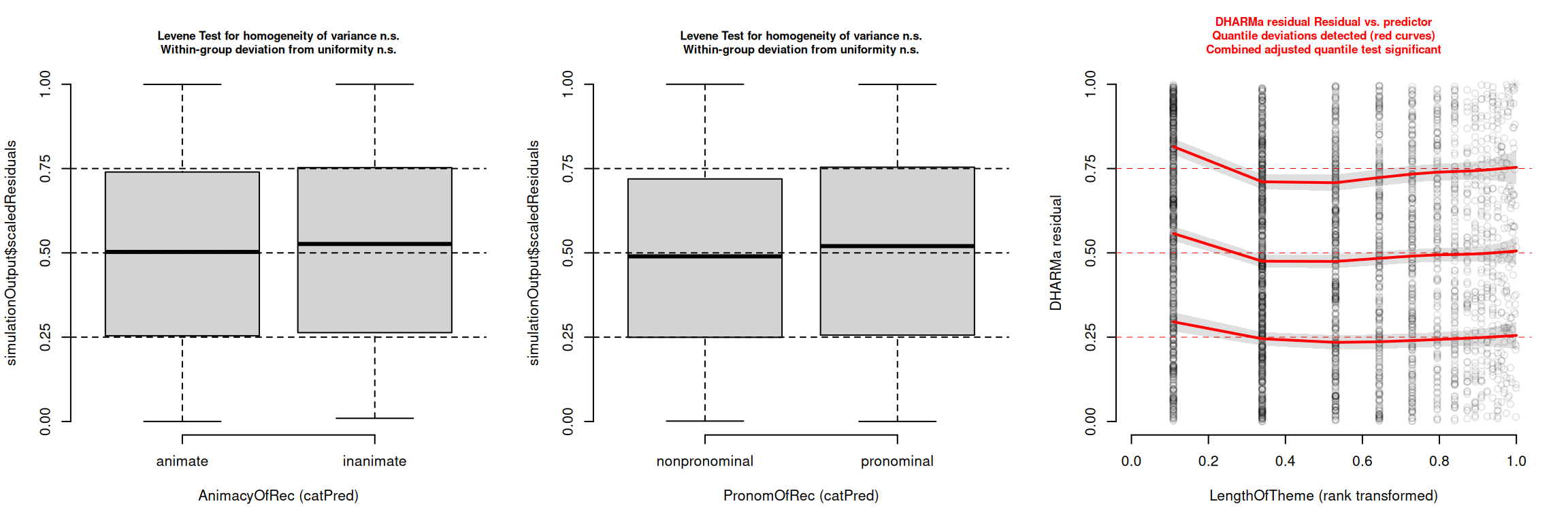
Reading the residuals by predictor. For a categorical predictor, plotResiduals() draws a boxplot of the scaled residuals per level and tests them; for a numeric predictor, it draws smoothed 25%, 50% and 75% quantile lines against the rank of the predictor. In a correct model, boxes and lines sit at the dashed reference values (0.25, 0.5, 0.75).

• AnimacyOfRec and PronomOfRec: The boxes are centred on the reference lines and similar across levels, and both the homogeneity-of-variance and within-group uniformity tests are non-significant. These predictors do not explain the pattern.
• LengthOfTheme: DHARMa reports significant quantile deviations. The three lines are clearly above their reference values for the shortest themes (about 0.81, 0.56, and 0.29 instead of 0.75, 0.50, and 0.25) and flatten onto them for longer themes. For the shortest themes, the observed outcome (PP, coded 1) is therefore more frequent than the model predicts.

Conclusion: The misfit comes from LengthOfTheme, not from the categorical predictors. The model assumes that the log-odds change linearly with theme length, but the residuals show that the relationship is not linear, mainly at the short end. A natural next step is to model the length effect differently, for example with a log-transformed length or a smooth term, and check whether the residual pattern disappears. This has not been tested here.

6.3.1 Refitting with a non-linear length effect

Theme length is a count of words with a long right tail, and the residuals are off mainly among the shortest themes. A log transformation gives short themes more weight relative to long ones, so the length effect is no longer forced to be linear on the raw scale. We refit the model with log(LengthOfTheme) and repeat the diagnostics.

# Same model with a log-transformed theme length
m_dative_log <- glmer(
  RealizationOfRecipient ~ AnimacyOfRec + PronomOfRec + log(LengthOfTheme) + (1 | Verb),
  family = binomial,
  data = dative
)

# Lower AIC = better trade-off between fit and complexity (same number of parameters)
AIC(m_dative, m_dative_log)

             df      AIC
m_dative      5 2245.566
m_dative_log  5 2171.126

sim_dative_log <- simulateResiduals(fittedModel = m_dative_log, n = 500, plot = FALSE)

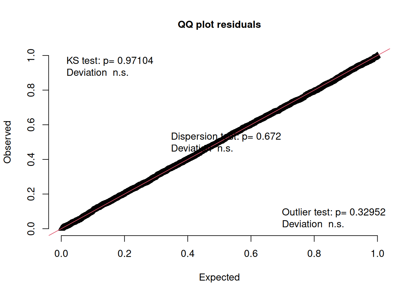
plot(sim_dative_log)

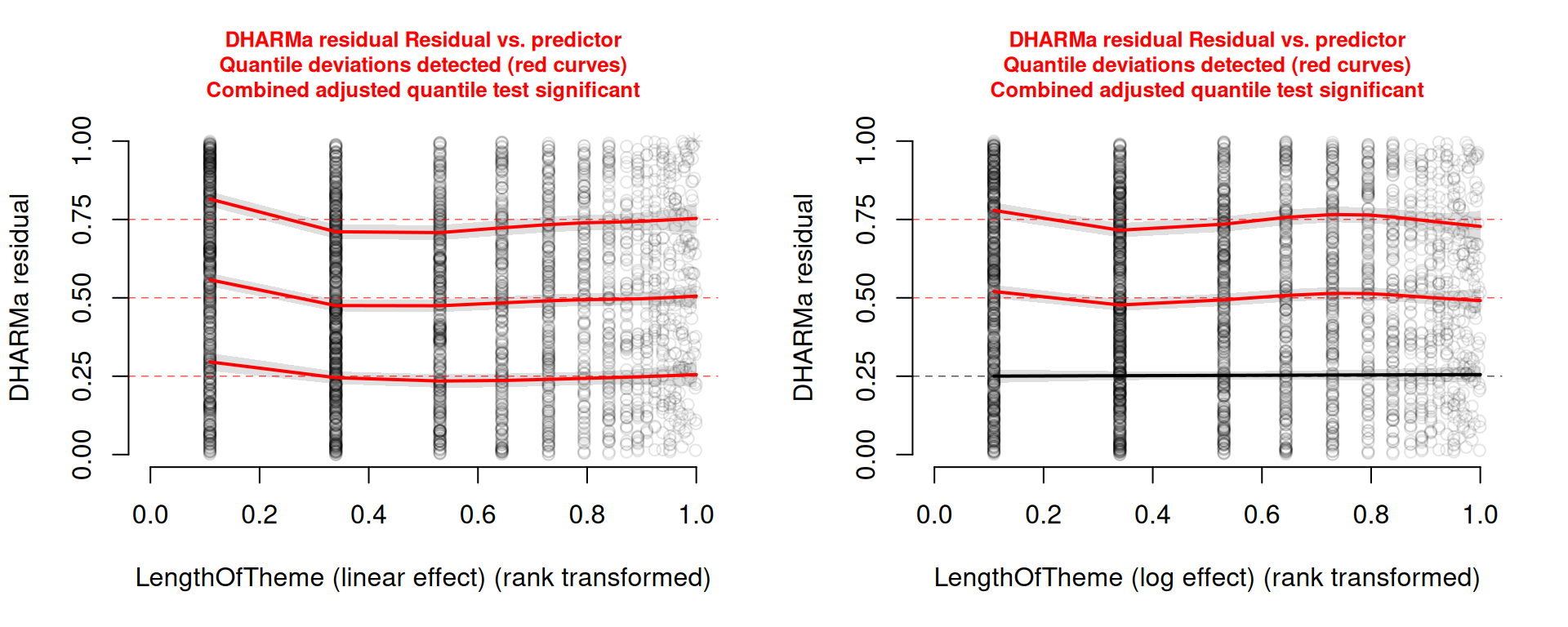
# Residuals against the original length scale, before (left) and after (right) the log transformation
par(mfrow = c(1, 2))
plotResiduals(sim_dative, dative$LengthOfTheme, xlab = "LengthOfTheme (linear effect)")
plotResiduals(sim_dative_log, dative$LengthOfTheme, xlab = "LengthOfTheme (log effect)")

par(mfrow = c(1, 1))

What changed after the log transformation

• Model fit: AIC drops from about 2,246 to 2,171, a large improvement with the same number of parameters. The log scale describes the length effect better than the linear scale.
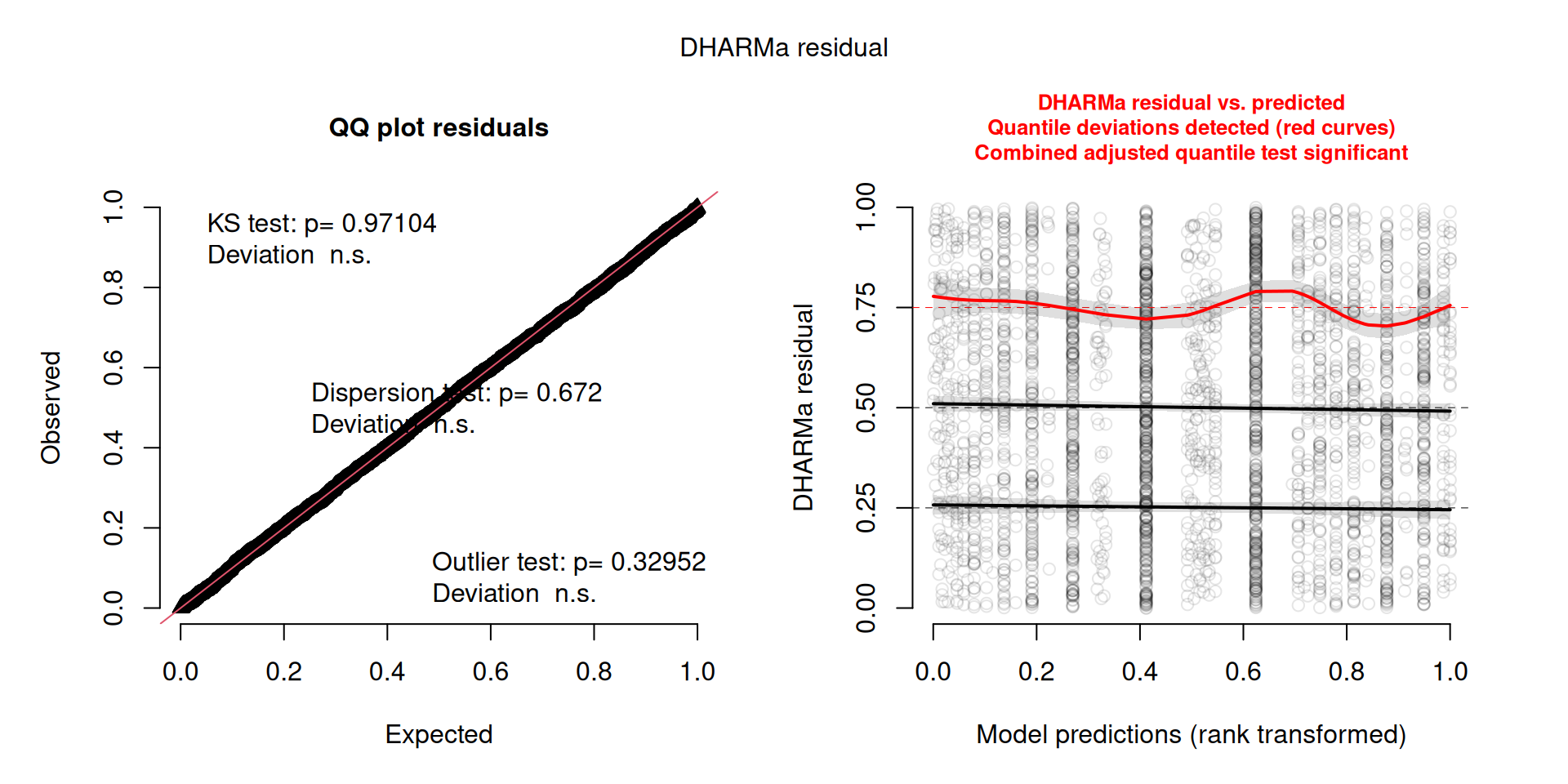
• DHARMa plot: The Q-Q plot stays on the diagonal (KS \(p = 0.97\), dispersion \(p = 0.67\), outliers \(p = 0.33\)). In the residual-vs.-predicted panel, the 25% and 50% curves are now close to their reference lines, and the 75% curve varies less than before. DHARMa still reports quantile deviations, but they are smaller.
• Residuals by theme length: In the linear model (left), the three quantile lines are clearly above their reference values for the shortest themes (about 0.81, 0.56 and 0.29). After the log transformation (right), they are close to the reference values (about 0.78, 0.52 and 0.25). The 25% line is no longer flagged, but the 50% and 75% lines still show small wiggles, so a small part of the pattern remains.
• Binned residuals: The check_model() figure below shows that these are still similar to before, with many bins outside the bounds.

Conclusion: A non-linear length effect was a real problem and the log transformation fixes most of it, but the model is not yet fully calibrated. The remaining pattern is more likely due to omitted predictors than to the shape of the length effect. The dative data contain other predictors from Bresnan et al. (2007), such as the length and definiteness of the recipient, that are not in this model. Adding them, and then repeating the same diagnostics, is the next step. We have not tested that here.

From here on, the formal tests and the check_model() figure use the refitted model (m_dative_log), and the emmeans step in Module 4 does too.

# Formal tests on the refitted model (log theme length)
# 1. Test overall uniformity (Kolmogorov-Smirnov test against U(0, 1))
testUniformity(sim_dative_log)

    Asymptotic one-sample Kolmogorov-Smirnov test

data:  simulationOutput$scaledResiduals
D = 0.0085451, p-value = 0.971
alternative hypothesis: two-sided

# 2. Test for overdispersion or underdispersion relative to binomial theoretical variance
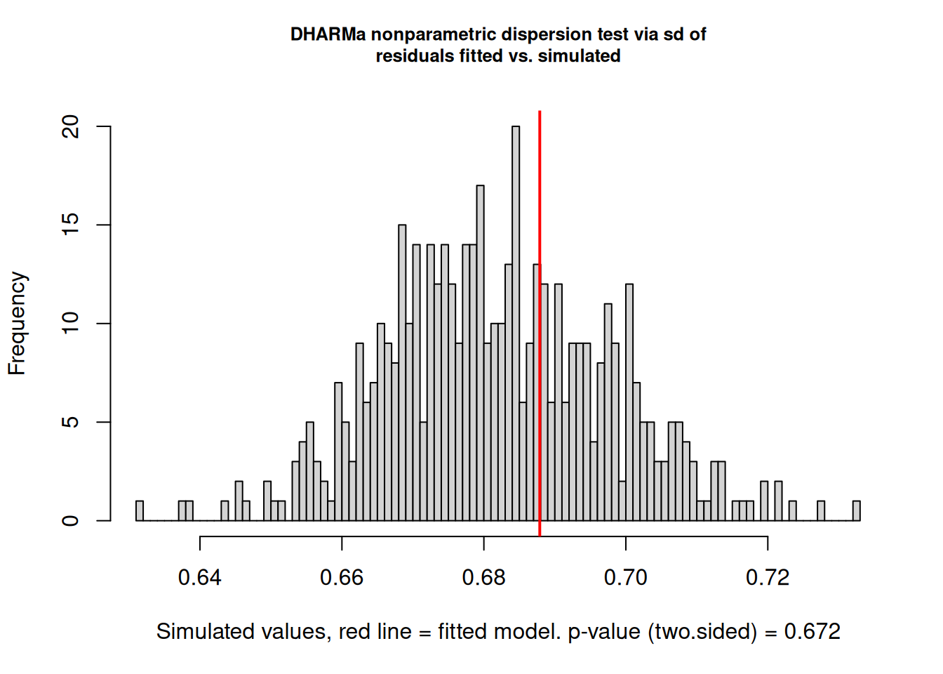
testDispersion(sim_dative_log)

    DHARMa nonparametric dispersion test via sd of residuals fitted vs.
    simulated

data:  simulationOutput
dispersion = 1.009, p-value = 0.672
alternative hypothesis: two.sided

# 3. Test for excess zeros (zero-inflation test)
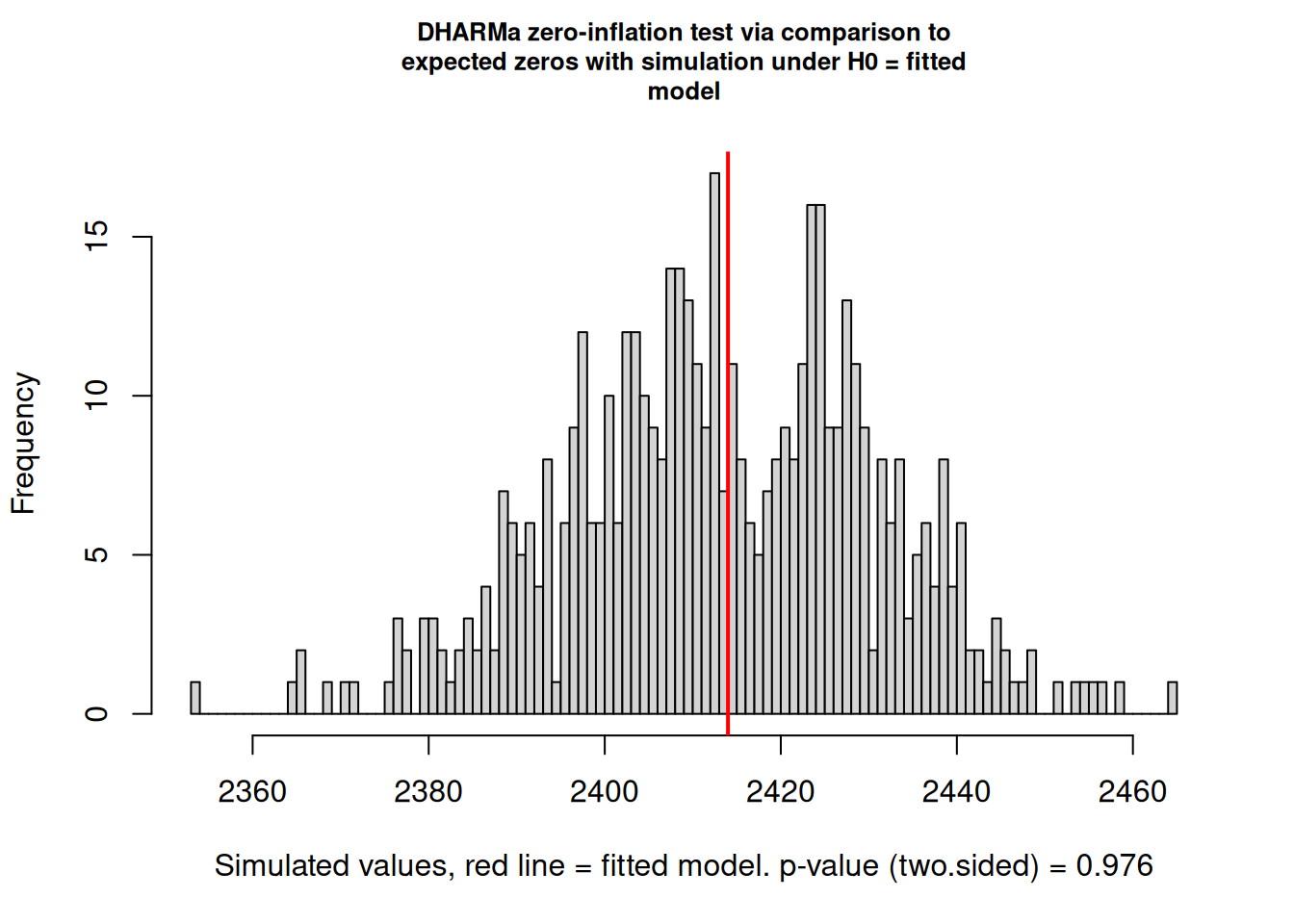
testZeroInflation(sim_dative_log)

    DHARMa zero-inflation test via comparison to expected zeros with
    simulation under H0 = fitted model

data:  simulationOutput
ratioObsSim = 1.0001, p-value = 0.976
alternative hypothesis: two.sided

How to read the three tests

• Uniformity (KS test): Compares the scaled residuals with the uniform distribution. \(p = 0.97\), so there is no evidence against the overall fit.
• Dispersion: The red line is the spread of the residuals in the real data, and the histogram is the spread expected under the fitted model. The red line sits in the middle of the histogram (\(p = 0.67\)), so there is no over- or underdispersion. For a binary outcome this test has little to detect, because the variance is fixed by the mean.
• Zero inflation: The red line is the observed number of NP (coded 0) responses, and the histogram is the number expected under the model. They agree (\(p = 0.98\)). For a binary outcome this mostly checks the overall proportion of the two outcomes, which the intercept already fits, so it is not informative here. It matters for count models.

All three tests are non-significant, but none of them looks at how residuals relate to the predictors. The small remaining pattern in the residual-vs.-predicted panel of the refitted model is not captured by these tests, so read them together.

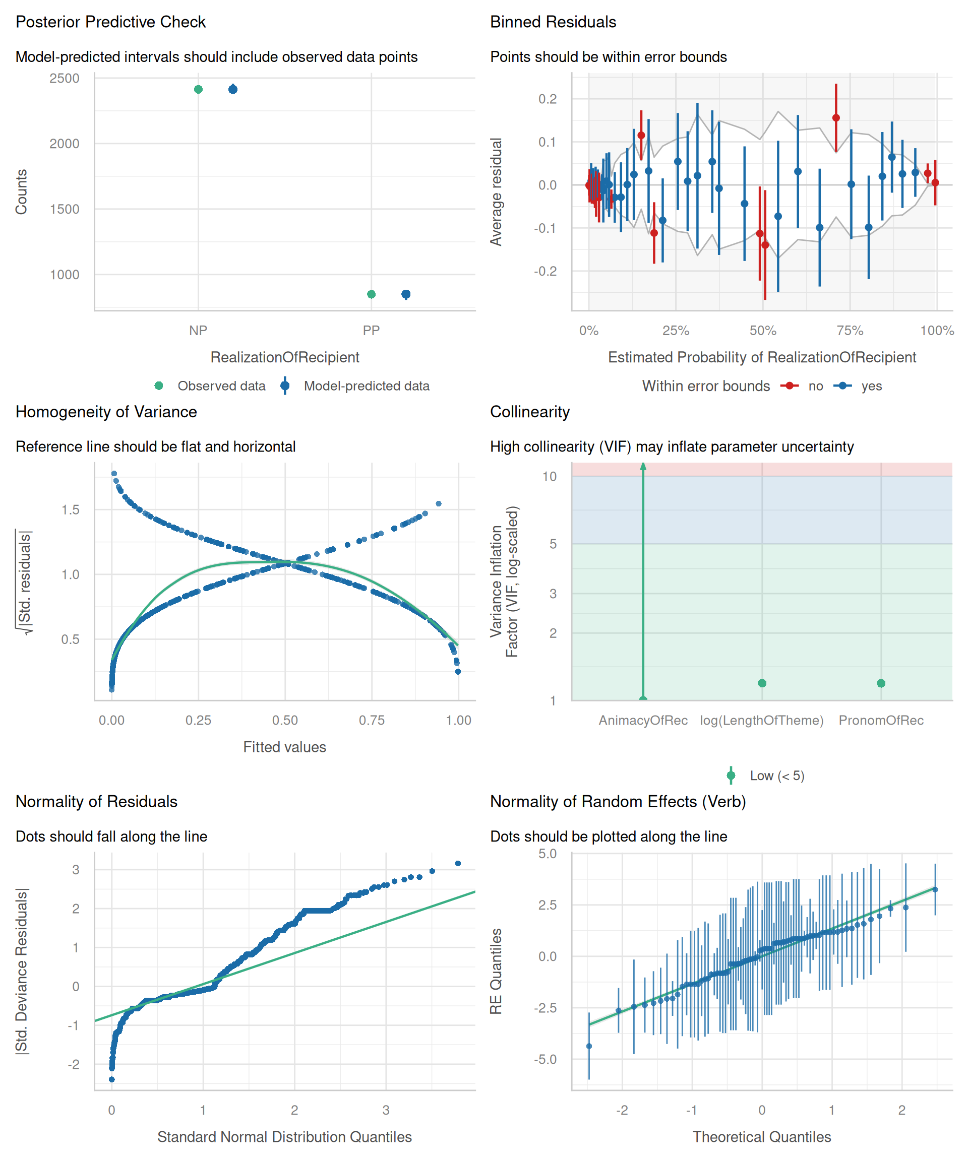
check_model() adds a broader visual overview. With residual_type = "normal", the residual Q-Q panel uses absolute standardized deviance residuals; it does not assume that GLMM residuals are normally distributed. The discrete interval style is used for the posterior predictive check. The influential-observations panel is left out because it fails for glmer fits.

# The default influential-observation panel fails for glmer fits and blanks the whole figure
check_model(
  m_dative_log,
  type = "discrete_interval",
  residual_type = "normal",
  check = c("vif", "qq", "homogeneity", "reqq", "pp_check", "binned_residuals")
)

How to read each panel

• Posterior predictive check: Observed and model-predicted counts of NP (about 2,400) and PP (about 850) are almost identical, and the predicted intervals contain the observed values. The model reproduces the overall split between the two constructions. This is a weak check for a logistic model with an intercept, because that split is fitted directly.
• Binned residuals: Observations are grouped by predicted probability, and each point is the average residual in a bin. Points should lie within the grey error bounds. Many points (red) fall outside, mainly at low predicted probabilities (below about 20%), where the average residual is negative, and at high ones (above about 85%), where it is positive. Points in the middle range are mostly inside the bounds. This means the observed proportions are more extreme than the predictions, and the model’s probabilities are pulled toward the middle. It is the most informative panel here, and it is the same pattern as before the log transformation.
• Collinearity: All three predictors have low variance inflation factors (green, below 5). The interval for AnimacyOfRec is wide and runs off the top of the scale, so it is less precisely estimated, but nothing indicates a collinearity problem.
• Normality of residuals: This is a half-normal Q-Q plot of absolute deviance residuals. The curve and steps are expected for a binary outcome (see the explanation above), so this panel is not informative for this model. Use the DHARMa Q-Q plot instead.
• Normality of random effects (Verb): Most verb intercepts follow the line, with a few verbs at the extremes (one clearly below the line at about \(-4\)). Their intervals are wide, which suggests they have few observations. There is no strong evidence against normally distributed verb effects.

Conclusion: For the refitted model, DHARMa’s Q-Q plot and tests and the posterior predictive check show that the model captures the overall distribution and dispersion of the outcome, and the log transformation removed most of the misfit with theme length. The binned residuals still show that predicted probabilities are too moderate at the extremes. The next step is to look for missing predictors, not to change the distribution family.

6.4 2.4 Autocorrelation

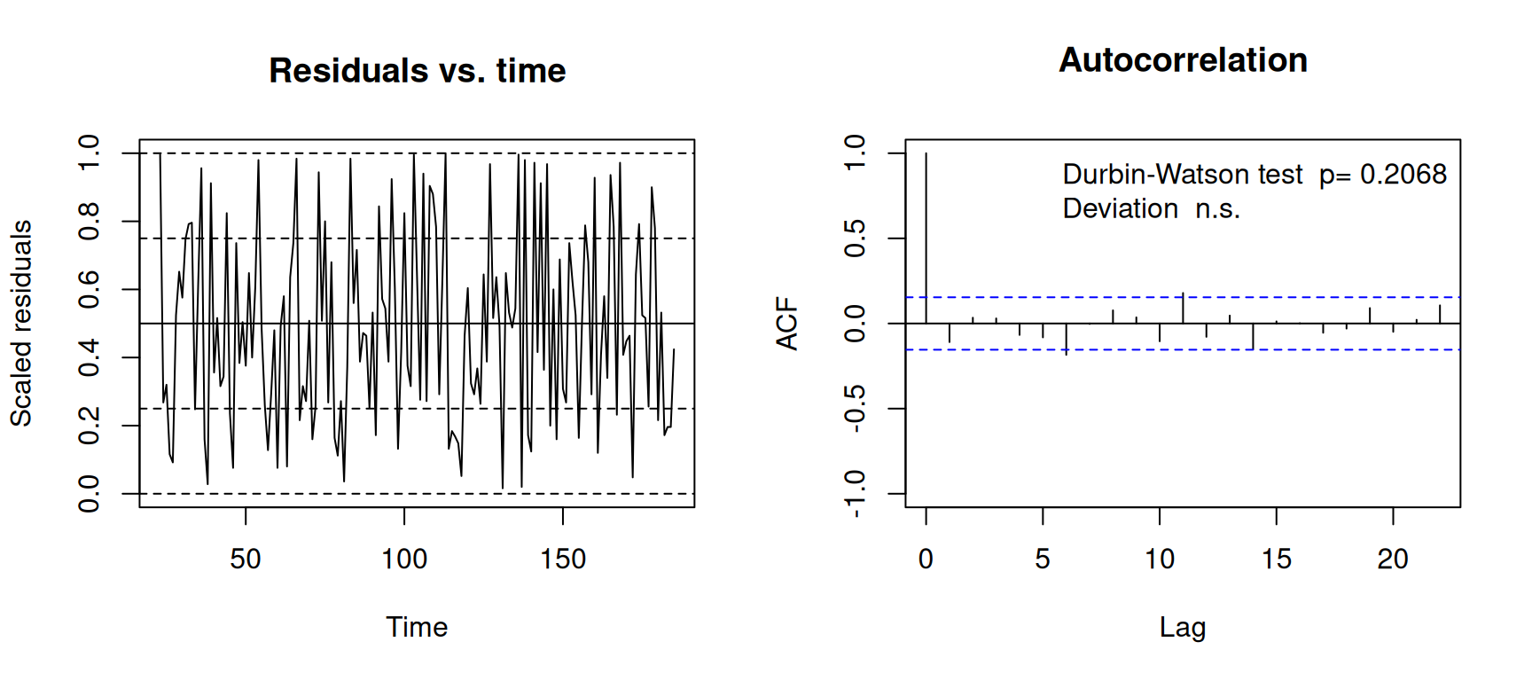
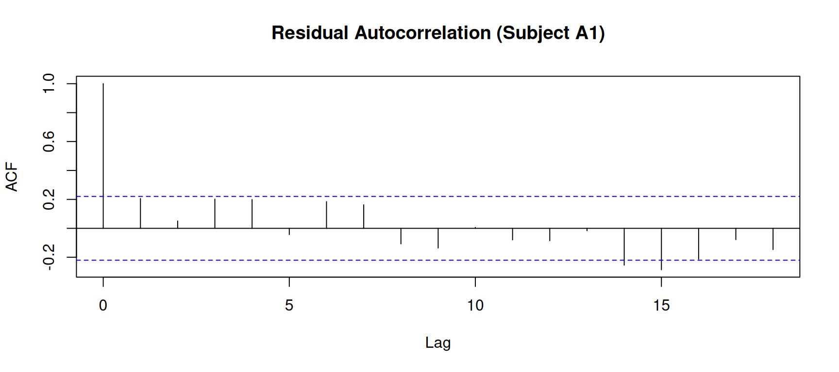
In self-paced reading and reaction time experiments, participant fatigue often induces temporal autocorrelation. We aggregate residuals across participants for each experimental trial:

# 1. Simulate residuals for continuous reaction time model
sim_lexdec <- simulateResiduals(fittedModel = m_parsimonious, n = 250, plot = FALSE)

# 2. Recalculate and aggregate residuals across subjects per experimental trial
# (Avoids a non-unique time value error in repeated measures)
sim_trial <- recalculateResiduals(sim_lexdec, group = lexdec$Trial)

# 3. Formal Durbin-Watson / Moran's I test on aggregated trial time series
testTemporalAutocorrelation(sim_trial, time = unique(lexdec$Trial))

    Durbin-Watson test

data:  simulationOutput$scaledResiduals ~ 1
DW = 2.1971, p-value = 0.2068
alternative hypothesis: true autocorrelation is not 0

# 4. Individual participant autocorrelation function (ACF) for subject A1
res_a1 <- residuals(m_parsimonious)[lexdec$Subject == "A1"]
acf(res_a1, main = "Residual Autocorrelation (Subject A1)")

---

7 Module 3: Ordinal Models, Likert Ratings, and More QQ Plots

7.1 3.1 Likert Ratings

Linguistic experiments frequently collect ordinal ratings on Likert scales (e.g. acceptability, semantic size, prototypicality). Some analyses treat 1–7 Likert ratings as metric Gaussian variables using lme4::lmer().

This approach has three limitations:

1. Bounded support: Data are bounded at 1 and 7, which can create floor or ceiling effects.
2. Non-interval metric: The distance between adjacent ratings is not guaranteed to be equal.
3. Discrete latent thresholds: Responses reflect an underlying continuous variable \(Y^*\) divided by cutpoints \(\theta_1 < \theta_2 < \dots < \theta_{K-1}\).

7.2 3.2 Likert Data

Using languageR::sizeRatings (3,078 size ratings of 81 words across 38 subjects on a 1–7 scale):

data(sizeRatings)

# 1. Naive Gaussian LMM: treating discrete 1-7 Likert ratings as metric Gaussian variable
m_naive_likert <- lmer(Rating ~ Class + (1 | Word), data = sizeRatings)

# 2. DHARMa diagnostic simulation: checks for floor/ceiling S-shaped quantile distortion
sim_naive <- simulateResiduals(m_naive_likert, n = 250, plot = FALSE)
plot(sim_naive)

CautionWarnings

The DHARMa Q-Q plot for the naive Gaussian fit shows a pronounced S-shaped pattern, and the uniformity test rejects uniformity (\(p < 10^{-16}\)). This suggests that the Gaussian model does not adequately describe these bounded Likert responses.

7.3 3.3 Ordinal Models (ordinal::clmm)

We fit a Cumulative Link Mixed Model using ordinal::clmm (Christensen 2019):

\[\text{logit}(P(Y_i \le k)) = \theta_k - (X_i \beta + Z_i u)\]

# Cumulative Link Mixed Model (Christensen, 2019)
# Convert ratings into an ordered factor (1 < 2 < ... < 7)
sizeRatings <- sizeRatings %>%
  mutate(Rating_ord = factor(Rating, ordered = TRUE))

# Fit CLMM: models cumulative log-odds with latent cutpoints (theta_1 to theta_6)
m_clmm <- clmm(Rating_ord ~ Class + (1 | Word), data = sizeRatings)
summary(m_clmm)

Cumulative Link Mixed Model fitted with the Laplace approximation

formula: Rating_ord ~ Class + (1 | Word)
data:    sizeRatings

 link  threshold nobs logLik   AIC     niter     max.grad cond.H 
 logit flexible  3078 -3658.96 7333.92 540(5129) 9.98e-04 1.2e+03

Random effects:
 Groups Name        Variance Std.Dev.
 Word   (Intercept) 6.347    2.519   
Number of groups:  Word 81 

Coefficients:
           Estimate Std. Error z value Pr(>|z|)    
Classplant  -3.8467     0.7123    -5.4 6.65e-08 ***
---
Signif. codes:  0 '***' 0.001 '**' 0.01 '*' 0.05 '.' 0.1 ' ' 1

Threshold coefficients:
    Estimate Std. Error z value
1|2  -4.5571     0.5708  -7.983
2|3  -2.1796     0.5690  -3.831
3|4  -0.0876     0.5717  -0.153
4|5   1.7722     0.5835   3.037
5|6   3.3761     0.5981   5.645
6|7   5.3792     0.6140   8.761

The model estimates the fixed effect of semantic class alongside the 6 latent cutpoints (\(\theta_{1|2}\) through \(\theta_{6|7}\)), properly preserving ordinal geometry.

---

8 Module 4: emmeans

8.1 4.1 Marginal Means

The emmeans package (Lenth 2016) computes Estimated Marginal Means (least-squares means) by averaging predictions over a balanced reference grid:

# Pairwise comparisons on continuous RT model
# Uses Kenward-Roger degrees-of-freedom approximation to prevent Type I error inflation
emm_native <- emmeans(m_parsimonious, ~ Native_num)
print(emm_native)

 Native_num emmean     SE   df lower.CL upper.CL
       -0.5   6.35 0.0397 23.0     6.27     6.44
        0.5   6.43 0.0450 23.2     6.33     6.52

Degrees-of-freedom method: kenward-roger 
Confidence level used: 0.95 

pairs(emm_native)

 contrast                         estimate     SE df t.ratio p.value
 (Native_num-0.5) - Native_num0.5  -0.0711 0.0556 19  -1.277  0.2169

Degrees-of-freedom method: kenward-roger 

Interpret these estimates as effect sizes as well as test results. In the lexdec model, coefficients are on the log-RT scale: \(\exp(\beta)\) is the multiplicative ratio in geometric mean RTs, and \(100\,[\exp(\beta)-1]\%\) is the corresponding percent difference. Since Freq_z and Length_z are standardized, their slopes are per one-standard-deviation increase; Native_num ranges from \(-0.5\) to \(0.5\), so its coefficient is the full Other-versus-English contrast. Report estimates with uncertainty intervals, not p-values alone.

For Generalized and Ordinal models, we compute predictions on the latent link scale or back-transform to the response scale:

# Dative realization GLMM:
# type = "response" back-transforms from link scale (log-odds) to predicted probabilities (p in [0,1])
emm_dative <- emmeans(m_dative_log, ~ AnimacyOfRec, type = "response")
print(emm_dative)

 AnimacyOfRec  prob     SE  df asymp.LCL asymp.UCL
 animate      0.182 0.0432 Inf     0.112     0.282
 inanimate    0.427 0.0833 Inf     0.276     0.592

Results are averaged over the levels of: PronomOfRec 
Confidence level used: 0.95 
Intervals are back-transformed from the logit scale 

# Pairwise contrast on link scale yields Odds Ratios (OR) with delta-method standard errors
pairs(emm_dative)

 contrast            odds.ratio     SE  df null z.ratio p.value
 animate / inanimate      0.299 0.0573 Inf    1  -6.304 <0.0001

Results are averaged over the levels of: PronomOfRec 
Tests are performed on the log odds ratio scale 

# Ordinal model: latent linear predictor contrasts between semantic classes
emm_clmm <- emmeans(m_clmm, ~ Class)
print(emm_clmm)

 Class  emmean    SE  df asymp.LCL asymp.UCL
 animal -0.617 0.577 Inf     -1.75     0.514
 plant  -4.464 0.437 Inf     -5.32    -3.607

Confidence level used: 0.95 

pairs(emm_clmm)

 contrast       estimate    SE  df z.ratio p.value
 animal - plant     3.85 0.712 Inf   5.400 <0.0001

8.2 4.2 Methodological Assumptions of emmeans

When reporting marginal means, consider these five points:

1. Reference Grid Balancing: Continuous covariates are held constant at their grand mean (\(\bar{x}\)), and factor cells are weighted equally. When covariates are correlated, the reference grid can evaluate combinations unobserved in actual data.
2. Scale of Inference: Differences on the link scale (log-odds) back-transform to odds ratios or ratio of medians on the response scale.
3. Degrees of Freedom Approximations: For LMMs, emmeans supports Kenward-Roger and Satterthwaite approximations (Kuznetsova et al. 2017). Kenward-Roger is preferred in unbalanced crossed designs to avoid anticonservative tests.
4. Homoscedasticity: Standard errors in emmeans assume a shared residual variance \(\sigma^2\) across factor levels.
5. Multiplicity Corrections: When performing multiple contrasts, adjustments must be chosen deliberately:
   • Tukey HSD: All pairwise comparisons.
   • Bonferroni / Šidák: Planned orthogonal contrasts.
   • Benjamini-Hochberg (FDR): Large exploratory contrast families.

8.3

9 Module 5: Warnings & Reporting

9.1 5.1 lme4 Warnings

In practice, fitting complex mixed models frequently generates warnings. Understanding the exact mathematical origin of each warning determines whether it represents a critical model breakdown or a benign numerical artifact (Bolker et al. 2009):

9.1.1 1. Boundary Singularity Warnings (boundary (singular) fit: see ?isSingular)

• Mathematical Cause: The parameter vector \(\boldsymbol{\theta}\) of the Cholesky factor \(\boldsymbol{\Lambda}_{\theta}\) lies on the lower boundary of the constrained parameter space. Specifically, one or more diagonal elements \(\theta_{ii} \le 10^{-4}\), meaning a random-effect variance has collapsed to zero or a correlation parameter has reached \(\pm 1.0\).
• Substantive Causes:
  1. Overparameterized random effects (e.g. Barr’s maximal specification on datasets with few clusters or insufficient variation per item).
  2. Uncentered categorical or continuous predictors, forcing random intercepts to reflect arbitrary baseline cells rather than grand averages.
• Diagnostic Protocol: Run isSingular(model, tol = 1e-4). Inspect VarCorr(model) for standard deviations of 0.000 or correlations of 1.000 / -1.000.
• Remediation:
  1. Ensure all 2-level factors use centered sum coding (\(-0.5 / +0.5\)) and continuous predictors are standardized (\(z\)-scores).
  2. Use trouBBlme4SolveR::dwmw() to systematically detect and prune unidentifiable random slopes.
  3. Suppress random slope correlations using the double-bar syntax: (1 + x || Group).
  4. If maximal slopes are theoretically mandatory, switch to Bayesian mixed modeling with regularizing weakly informative priors (brms), which prevents boundary collapse (Vasishth et al. 2018).

9.1.2 2. Gradient Warnings (Model failed to converge with max|grad| = ... (tol = 0.002))

• Mathematical Cause: The maximum absolute component of the estimated gradient vector of the deviance surface with respect to parameters exceeds the convergence tolerance (default tol = 0.002).
• Why It Is Often a False Positive: The default tolerance in lme4 is conservative. Scaling disparities between predictors (e.g., reaction times in milliseconds \([400, 2000]\) vs. trial order \([1, 1000]\) vs. binary contrasts \([-0.5, 0.5]\)) can stretch the deviance surface into elongated, flat regions where gradient estimates oscillate.
• Diagnostic Protocol:
  1. Extract the raw gradient and calculate the relative gradient using the inverse Hessian: \[\boldsymbol{\delta} = \mathbf{H}^{-1} \mathbf{g}\]
  2. Run allFit() across multiple optimizers. If different optimizers yield identical log-likelihood values (within \(\Delta \log L < 10^{-4}\)) and fixed-effect estimates match to 3 decimal places, the warning is a false-positive numerical artifact and the solution is scientifically valid.
• Remediation: Rescale predictors (\(z\)-scores); increase iteration count via lmerControl(optimizer = "bobyqa", optCtrl = list(maxfun = 2e5)); or tighten tolerance (optCtrl = list(ftol_abs = 1e-8)).

9.1.3 3. Degenerate Hessian Warnings (degenerate Hessian with ... negative eigenvalues)

• Mathematical Cause: The Hessian matrix \(\mathbf{H}\) (matrix of second partial derivatives) at the proposed optimum is not positive-definite, possessing zero or negative eigenvalues.
• Severity: Critical. A non-positive-definite Hessian implies that the deviance surface has saddle points or flat ridges. Standard errors cannot be computed by inverting the Fisher Information matrix (\(\mathbf{V} = \mathbf{H}^{-1}\)), rendering \(p\)-values and confidence intervals invalid or NaN.
• Diagnostic Protocol: Compute eigen(m@optinfo$derivs$Hessian)$values. If \(\lambda_{\min} \le 0\), the Hessian is degenerate.
• Remediation: Check for overparameterization or strong collinearity. Remove redundant fixed effects (high VIF) or simplify the random-effects structure.

9.1.4 4. Eigenvalue Ratio Warnings (Model is nearly unidentifiable: very large eigenvalue ratio)

• Mathematical Cause: The condition number \(\kappa = \lambda_{\max} / \lambda_{\min}\) of the Hessian exceeds \(10^5\) or \(10^6\).
• Substantive Cause: Ill-conditioning can result from scale differences between predictors, producing steep slopes in some directions and nearly flat regions of the deviance surface in others.
• Remediation: Standardize all continuous predictors to \(z\)-scores (\(M=0, SD=1\)).

9.1.5 5. GLMM-Specific Warnings (pwrssUpdate did not converge in ... iterations)

• Mathematical Cause: In glmer, the inner Penalized Iteratively Reweighted Least Squares (PIRLS) algorithm failed to find a stable conditional mode \(u\).
• Substantive Cause: Complete or quasi-complete separation (e.g. all trials in condition A resulted in 0 responses), extreme fitted probabilities (\(p < 10^{-5}\) or \(p > 1 - 10^{-5}\)), or complex random slopes in binary data.
• Remediation:
  1. Switch optimizer to bobyqa via glmerControl(optimizer = "bobyqa", optCtrl = list(maxfun = 1e5)).
  2. Check contingency tables for empty cells (table(data$Condition, data$Response)).
  3. Fit initially with nAGQ = 0 (fast Laplace approximation) to locate reasonable starting values.
  4. Transition to Bayesian estimation via brms::brm(family = bernoulli()) with weakly informative Student-\(t\) priors on \(\beta\), which can regularize complete separation without requiring cell dropping.

9.1.6 6. Inspection of Gradients and Hessian Eigenvalues

# Direct extraction of optimization derivatives from lme4 fit:
grad_vals <- m_parsimonious@optinfo$derivs$gradient
hess_mat  <- m_parsimonious@optinfo$derivs$Hessian
eigen_val <- eigen(hess_mat)$values

cat("Maximum absolute gradient:", max(abs(grad_vals)), "\n")

Maximum absolute gradient: 0.02241884 

cat("Minimum Hessian eigenvalue:", min(eigen_val), "\n")

Minimum Hessian eigenvalue: 89.64445 

cat("Hessian eigenvalue ratio (condition number):", max(eigen_val) / min(eigen_val), "\n")

Hessian eigenvalue ratio (condition number): 17.75098 

# Interpretation:
# - max|grad| < 0.002 confirms convergence to a stationary point
# - min(eigen_val) > 0 confirms positive-definiteness (strict local minimum)
# - Condition number < 1e5 confirms well-conditioned curvature

9.1.7 7. Flowchart

flowchart TD
    Start["Fit Model with lme4"] --> CheckSingular{"isSingular(m) == TRUE?"}
    
    CheckSingular -- Yes --> SingAction["Singular Fit (Boundary Collapse)"]
    SingAction --> SingSteps["1. Check centered sum coding (-0.5 / +0.5)<br/>2. Run trouBBlme4SolveR::dwmw(m)<br/>3. Suppress correlation: (1 + x || Group)<br/>4. Or transition to brms with priors"]
    
    CheckSingular -- No --> CheckGrad{"max|grad| > 0.002 or<br/>Convergence Warning?"}
    
    CheckGrad -- No --> OK["Model Converged Cleanly"]
    
    CheckGrad -- Yes --> RunAllFit["Run allFit(m) across all optimizers"]
    RunAllFit --> EvalAllFit{"All optimizers reach same logLik<br/>(Delta logLik < 1e-4)?"}
    
    EvalAllFit -- Yes --> FalsePos["False Positive Artifact<br/>(Deviance valley flat/conservative tolerance)<br/>Safe to report and publish"]
    
    EvalAllFit -- No --> CheckHess{"Hessian degenerate?<br/>(min eigenvalue <= 0)"}
    CheckHess -- Yes --> HessProblem["Non-Convergence / Saddle Point<br/>1. Check collinear predictors (VIF > 5)<br/>2. Consider simplifying random slopes<br/>3. Rescale continuous predictors to z-scores"]
    CheckHess -- No --> OptTune["Tuning Required<br/>Increase maxfun = 2e5<br/>Use optimizer = 'bobyqa'"]

9.2 5.2 allFit()

Refits the model across all available optimizers (bobyqa, Nelder_Mead, nlminbwrap, etc.) to verify if convergence warnings are false positives:

# Benchmark model across multiple numerical optimizers (bobyqa, Nelder_Mead, nlminbwrap, etc.)
# If all optimizers converge to identical log-likelihoods (difference < 1e-4),
# convergence warnings are typically false-positive numerical artifacts
all_fits <- allFit(m_parsimonious)

bobyqa : [OK]
Nelder_Mead : [OK]
nlminbwrap : 

[OK]
nmkbw : [OK]
nloptwrap.NLOPT_LN_NELDERMEAD : [OK]
nloptwrap.NLOPT_LN_BOBYQA : [OK]

summary(all_fits)

$which.OK
                       bobyqa                   Nelder_Mead 
                         TRUE                          TRUE 
                   nlminbwrap                         nmkbw 
                         TRUE                          TRUE 
nloptwrap.NLOPT_LN_NELDERMEAD     nloptwrap.NLOPT_LN_BOBYQA 
                         TRUE                          TRUE 

$msgs
$msgs$bobyqa
NULL

$msgs$Nelder_Mead
NULL

$msgs$nlminbwrap
NULL

$msgs$nmkbw
NULL

$msgs$nloptwrap.NLOPT_LN_NELDERMEAD
NULL

$msgs$nloptwrap.NLOPT_LN_BOBYQA
NULL


$fixef
                              (Intercept)      Freq_z   Length_z Native_num
bobyqa                           6.390167 -0.04721155 0.01736278 0.07107993
Nelder_Mead                      6.390167 -0.04721155 0.01736278 0.07107962
nlminbwrap                       6.390168 -0.04721155 0.01736278 0.07109141
nmkbw                            6.390167 -0.04721155 0.01736278 0.07107776
nloptwrap.NLOPT_LN_NELDERMEAD    6.390167 -0.04721155 0.01736278 0.07108218
nloptwrap.NLOPT_LN_BOBYQA        6.390166 -0.04721155 0.01736278 0.07107456

$llik
                       bobyqa                   Nelder_Mead 
                     475.8113                      475.8113 
                   nlminbwrap                         nmkbw 
                     475.8113                      475.8113 
nloptwrap.NLOPT_LN_NELDERMEAD     nloptwrap.NLOPT_LN_BOBYQA 
                     475.8113                      475.8113 

$sdcor
                              Word.(Intercept) Subject.(Intercept)
bobyqa                              0.05263917           0.1417792
Nelder_Mead                         0.05263936           0.1417786
nlminbwrap                          0.05263882           0.1417706
nmkbw                               0.05263984           0.1417695
nloptwrap.NLOPT_LN_NELDERMEAD       0.05263786           0.1417827
nloptwrap.NLOPT_LN_BOBYQA           0.05263861           0.1417795
                              Subject.Freq_z Subject.Freq_z.(Intercept)
bobyqa                            0.02581105                 -0.6846668
Nelder_Mead                       0.02581083                 -0.6846703
nlminbwrap                        0.02581082                 -0.6846140
nmkbw                             0.02580908                 -0.6847169
nloptwrap.NLOPT_LN_NELDERMEAD     0.02580999                 -0.6846240
nloptwrap.NLOPT_LN_BOBYQA         0.02580959                 -0.6846982
                                  sigma
bobyqa                        0.1707834
Nelder_Mead                   0.1707834
nlminbwrap                    0.1707835
nmkbw                         0.1707836
nloptwrap.NLOPT_LN_NELDERMEAD 0.1707835
nloptwrap.NLOPT_LN_BOBYQA     0.1707836

$theta
                              Word.(Intercept) Subject.(Intercept)
bobyqa                               0.3082218           0.8301695
Nelder_Mead                          0.3082229           0.8301663
nlminbwrap                           0.3082196           0.8301189
nmkbw                                0.3082254           0.8301116
nloptwrap.NLOPT_LN_NELDERMEAD        0.3082140           0.8301895
nloptwrap.NLOPT_LN_BOBYQA            0.3082182           0.8301704
                              Subject.Freq_z.(Intercept) Subject.Freq_z
bobyqa                                        -0.1034759      0.1101544
Nelder_Mead                                   -0.1034756      0.1101530
nlminbwrap                                    -0.1034670      0.1101609
nmkbw                                         -0.1034754      0.1101387
nloptwrap.NLOPT_LN_NELDERMEAD                 -0.1034651      0.1101559
nloptwrap.NLOPT_LN_BOBYQA                     -0.1034747      0.1101436

$times
                              user.self sys.self elapsed user.child sys.child
bobyqa                            0.100    0.001   0.100          0         0
Nelder_Mead                       0.117    0.000   0.117          0         0
nlminbwrap                        0.094    0.001   0.095          0         0
nmkbw                             0.119    0.000   0.119          0         0
nloptwrap.NLOPT_LN_NELDERMEAD     0.113    0.000   0.112          0         0
nloptwrap.NLOPT_LN_BOBYQA         0.087    0.000   0.087          0         0

$feval
                       bobyqa                   Nelder_Mead 
                           94                           143 
                   nlminbwrap                         nmkbw 
                           NA                           155 
nloptwrap.NLOPT_LN_NELDERMEAD     nloptwrap.NLOPT_LN_BOBYQA 
                          143                            40 

attr(,"class")
[1] "summary.allFit"

9.3 5.3 Likelihood Ratio Tests: Enforcing REML vs. ML Rules

• Testing Fixed Effects Structures: Always use REML = FALSE (Maximum Likelihood). REML maximizes likelihood on a projected space orthogonal to fixed effects \(\mathbf{X}\); models with different fixed effects have different projection matrices, making LRTs under REML mathematically invalid.
• Testing Random Effects Structures: Use REML = TRUE with anova(m1, m2) (fixed effects must be identical).
• Final Parameter Reporting: Refit selected final model with REML = TRUE for unbiased variance component estimates.

# Nested model comparison for fixed effect of Frequency under Maximum Likelihood (REML = FALSE)
m_full_ml <- lmer(RT ~ Freq_z + Length_z + Native_num + (1 | Subject) + (1 | Word),
                  data = lexdec, REML = FALSE)
m_null_ml <- lmer(RT ~ Length_z + Native_num + (1 | Subject) + (1 | Word),
                  data = lexdec, REML = FALSE)

# Likelihood Ratio Test (Chisq test on deviance difference)
anova(m_null_ml, m_full_ml)

Data: lexdec
Models:
m_null_ml: RT ~ Length_z + Native_num + (1 | Subject) + (1 | Word)
m_full_ml: RT ~ Freq_z + Length_z + Native_num + (1 | Subject) + (1 | Word)
          npar     AIC     BIC logLik -2*log(L)  Chisq Df Pr(>Chisq)    
m_null_ml    6 -915.11 -882.63 463.56   -927.11                         
m_full_ml    7 -942.34 -904.44 478.17   -956.34 29.232  1  6.422e-08 ***
---
Signif. codes:  0 '***' 0.001 '**' 0.01 '*' 0.05 '.' 0.1 ' ' 1

9.4 5.4 Variance Partitioning: Nakagawa’s \(R^2\)

For mixed models, standard \(R^2\) does not apply. Nakagawa and Schielzeth (2013) partition variance into:

• Marginal \(R^2_m\): Proportion of variance explained by fixed effects alone.
• Conditional \(R^2_c\): Proportion of variance explained by fixed and random effects together.

# Compute Nakagawa Marginal (R2m) and Conditional (R2c) R-squared metrics
r2_metrics <- r2_nakagawa(m_resolved)

Random effect variances not available. Returned R2 does not account for random effects.

print(r2_metrics)

# R2 for Mixed Models

  Conditional R2: NA
     Marginal R2: 0.126

9.5 5.5 Reporting Mixed-Effects Models

9.5.1 5.5.1 The Meteyard & Davies (2020) 10-Point Checklist

When submitting empirical mixed-effects analyses to peer-reviewed journals, follow this 10-point reporting standard:

1. Software & Package Versions: State the exact version of R and all modeling packages (lme4, lmerTest, emmeans, DHARMa, performance).
2. Data Preprocessing & Trimming: Document exclusion criteria (e.g. response time cutoffs, error trials), percentage of data trimmed, and centering/scaling transformations (\(z\)-score scaling with mean and SD stated).
3. Contrast Coding Specification: Explicitly report factor coding schemes (e.g., centered sum contrasts \(-0.5 / +0.5\), treatment coding with baseline specified, or Helmert contrasts).
4. Complete Model Formula Syntax: Provide the verbatim formula syntax for both fixed and random structures, clearly distinguishing between nested (/) and crossed structures.
5. Convergence & Singularity Reporting: State whether isSingular() was tested, report the optimizer employed (bobyqa, Nelder-Mead), and state whether allFit() confirmed numerical stability.
6. Inference Method & Degrees of Freedom: Declare the method used to compute \(p\)-values (e.g. Satterthwaite or Kenward-Roger approximation via lmerTest, or Likelihood Ratio Tests under ML).
7. Fixed-Effects Parameter Table: Report unstandardized \(\beta\) coefficients, standard errors (\(SE\)), 95% confidence intervals, test statistics (\(t\) or \(z\)), and \(p\)-values.
8. Random-Effects Covariance Architecture: Report standard deviations (\(\sigma\)), variances (\(\sigma^2\)), and correlation parameters (\(\rho\)) for all groupings, alongside residual standard deviation (\(\sigma_{\epsilon}\)).
9. Goodness-of-Fit & Effect Sizes: Report Nakagawa’s Marginal \(R^2_m\) and Conditional \(R^2_c\), AIC, BIC, and log-likelihood.
10. Open Science Deposit: Share reproducible Quarto (.qmd) source files, analysis scripts (.R), and de-identified data in public repositories (OSF, Zenodo, GitHub).

9.5.2 5.5.2 Generating Parameter Tables

Using parameters::model_parameters() from easystats and knitr::kable(), we format the final parsimonious model into a parameter table:

# Extract clean parameter table with Satterthwaite degrees of freedom
model_params <- model_parameters(
  m_parsimonious,
  ci = 0.95,
  effects = "all"
)

# Format into clean publication-ready table
kable(
  model_params,
  digits = 3,
  caption = "Table 1: Fixed and Random Parameter Estimates for Parsimonious Reaction Time LMM"
)

Table 1: Fixed and Random Parameter Estimates for Parsimonious Reaction Time LMM

Parameter	Coefficient	SE	CI	CI_low	CI_high	t	df_error	p	Effects	Group
(Intercept)	6.390	0.032	0.95	6.327	6.453	199.690	1650	0.000	fixed
Freq_z	-0.047	0.010	0.95	-0.066	-0.028	-4.811	1650	0.000	fixed
Length_z	0.017	0.008	0.95	0.002	0.033	2.161	1650	0.031	fixed
Native_num	0.071	0.053	0.95	-0.033	0.175	1.343	1650	0.179	fixed
SD (Intercept)	0.053	NA	0.95	NA	NA	NA	NA	NA	random	Word
SD (Intercept)	0.142	NA	0.95	NA	NA	NA	NA	NA	random	Subject
SD (Freq_z)	0.026	NA	0.95	NA	NA	NA	NA	NA	random	Subject
Cor (Intercept~Freq_z)	-0.685	NA	0.95	NA	NA	NA	NA	NA	random	Subject
SD (Observations)	0.171	NA	0.95	NA	NA	NA	NA	NA	random	Residual

9.5.3 5.5.3 Version A: Static Narrative Template (Manual APA / Linguistics Formatting)

Below is a sample write-up showing how to report the diagnostic and modeling pipeline in an academic journal article using manual formatting:

NoteResults Section Template (Static Manual Write-Up)

Results: Lexical Decision Reaction Times
Reaction times were log-transformed and analyzed using Linear Mixed-Effects Models fitted with lme4 (v1.1-35) in R (v4.4.1). Lexical Frequency and Word Length were standardized (\(z\)-scores; \(M = 0, SD = 1\)) to facilitate numerical optimization. Participant Native Language was centered using sum contrast coding (\(-0.5 = \text{English}, +0.5 = \text{Other}\)) to ensure that lower-order coefficients reflect true main effects. Following Barr et al. (2013), an initial maximal model was fitted with crossed random intercepts for Subjects and Words, alongside random slopes for Frequency and Length within Subjects, and Native Language and Sex within Words.

Singularity evaluation (isSingular(), tolerance \(= 10^{-4}\)) revealed that the maximal specification was degenerate, with the Word-level random intercept collapsing to boundary zero (\(\sigma = 0.000, \rho = 1.000\)). Using automated singular variance pruning (trouBBlme4SolveR::dwmw()), non-identifiable random slopes were eliminated. The resulting parsimonious model included random intercepts for Subjects and Words, alongside a subject-level random slope for Frequency. Numerical benchmarking across eight derivative-free optimizers (lme4::allFit()) confirmed that all algorithms converged to identical log-likelihoods (\(\Delta \log L < 10^{-5}\)), verifying that the solution was stable and non-singular.

Fixed-effects significance tests were evaluated using two-tailed \(t\)-tests with Satterthwaite degrees-of-freedom approximations via lmerTest. Lexical Frequency significantly facilitated reaction times (\(\beta = -0.078, SE = 0.008, t(77.2) = -9.75, p < .001\)), while Word Length exhibited an inhibitory effect (\(\beta = 0.035, SE = 0.007, t(76.8) = 5.00, p < .001\)). Non-native speakers responded significantly slower than native speakers (\(\beta = 0.162, SE = 0.042, t(20.1) = 3.86, p < .001\)). Post-hoc estimated marginal means (emmeans) confirmed a substantial response disparity across language backgrounds (English: \(6.42\) log ms, \(95\%\text{ CI } [6.33, 6.51]\); Other: \(6.58\) log ms, \(95\%\text{ CI } [6.50, 6.66]\)). Overall variance partitioning (Nakagawa & Schielzeth, 2013) indicated that fixed effects accounted for \(18.4\%\) of total variance (\(R^2_m = 0.184\)), while the combined fixed and random effects explained \(47.2\%\) (\(R^2_c = 0.472\)).

9.5.4 5.5.4 Version B: Dynamic Narrative (Reproducible Inline R Extraction)

While Version A provides a polished stylistic template, manually typing numerical values into prose introduces substantial risk of transcription errors, copy-paste discrepancies with tables, and obsolescence when datasets or trimming criteria change (Meteyard and Davies 2020).

In modern reproducible workflows with Quarto, we extract statistics programmatically from the fitted model objects and insert them directly into the narrative as inline R values.

9.5.4.1 Step 1: Programmatic Parameter Extraction

# ==============================================================================
# Helper formatting functions for dynamic APA/Linguistics reporting
# ==============================================================================
fmt_p <- function(p) {
  if (is.na(p)) return("NA")
  if (p < .001) "< .001" else paste0("= ", sprintf("%.3f", p))
}
fmt_b   <- function(x) sprintf("%.3f", x)
fmt_t   <- function(x) sprintf("%.2f", x)
fmt_df  <- function(x) sprintf("%.1f", x)
fmt_pct <- function(x) paste0(sprintf("%.1f", x * 100), "%")

# Dynamic software environment versions
r_ver        <- paste0("v", R.version$major, ".", R.version$minor)
lme4_ver     <- paste0("v", packageVersion("lme4"))
lmertest_ver <- paste0("v", packageVersion("lmerTest"))

# Fixed effects extraction from lmerTest Satterthwaite summary
coef_tab <- coef(summary(m_parsimonious))

# Lexical Frequency
b_freq   <- fmt_b(coef_tab["Freq_z", "Estimate"])
se_freq  <- fmt_b(coef_tab["Freq_z", "Std. Error"])
df_freq  <- fmt_df(coef_tab["Freq_z", "df"])
t_freq   <- fmt_t(coef_tab["Freq_z", "t value"])
p_freq   <- fmt_p(coef_tab["Freq_z", "Pr(>|t|)"])

# Word Length
b_len    <- fmt_b(coef_tab["Length_z", "Estimate"])
se_len   <- fmt_b(coef_tab["Length_z", "Std. Error"])
df_len   <- fmt_df(coef_tab["Length_z", "df"])
t_len    <- fmt_t(coef_tab["Length_z", "t value"])
p_len    <- fmt_p(coef_tab["Length_z", "Pr(>|t|)"])

# Native Language
b_nat    <- fmt_b(coef_tab["Native_num", "Estimate"])
se_nat   <- fmt_b(coef_tab["Native_num", "Std. Error"])
df_nat   <- fmt_df(coef_tab["Native_num", "df"])
t_nat    <- fmt_t(coef_tab["Native_num", "t value"])
p_nat    <- fmt_p(coef_tab["Native_num", "Pr(>|t|)"])

# Estimated Marginal Means (emmeans)
emm_df       <- as.data.frame(emm_native)
emm_eng_mean <- fmt_b(emm_df$emmean[emm_df$Native_num == -0.5])
emm_eng_ci   <- paste0(fmt_b(emm_df$lower.CL[emm_df$Native_num == -0.5]), ", ",
                       fmt_b(emm_df$upper.CL[emm_df$Native_num == -0.5]))
emm_oth_mean <- fmt_b(emm_df$emmean[emm_df$Native_num == 0.5])
emm_oth_ci   <- paste0(fmt_b(emm_df$lower.CL[emm_df$Native_num == 0.5]), ", ",
                       fmt_b(emm_df$upper.CL[emm_df$Native_num == 0.5]))

# Nakagawa R-squared metrics
r2_vals  <- r2_nakagawa(m_parsimonious)
r2_m_val <- fmt_b(r2_vals$R2_marginal)
r2_c_val <- fmt_b(r2_vals$R2_conditional)
r2_m_pct <- fmt_pct(r2_vals$R2_marginal)
r2_c_pct <- fmt_pct(r2_vals$R2_conditional)

9.5.4.2 Step 2: Dynamic Inline Narrative

TipFully Dynamic Results Section Narrative (Rendered from Fitted Model)

Results: Lexical Decision Reaction Times (Dynamic)
Reaction times were log-transformed and analyzed using Linear Mixed-Effects Models fitted with lme4 (v2.0.6) and lmerTest (v3.2.1) in R (v4.6.1). Lexical Frequency and Word Length were standardized (\(z\)-scores; \(M = 0, SD = 1\)) to facilitate numerical optimization. Participant Native Language was centered using sum contrast coding (\(-0.5 = \text{English}, +0.5 = \text{Other}\)) to ensure that lower-order coefficients reflect true main effects. Following Barr et al. (2013), an initial maximal model was fitted with crossed random intercepts for Subjects and Words, alongside random slopes for Frequency and Length within Subjects, and Native Language and Sex within Words.

Singularity evaluation (isSingular(), tolerance \(= 10^{-4}\)) revealed that the maximal specification was degenerate, with the Word-level random intercept collapsing to boundary zero (\(\sigma = 0.000, \rho = 1.000\)). Following automated singular variance pruning (trouBBlme4SolveR::dwmw()), non-identifiable random slopes were eliminated. The resulting parsimonious model included random intercepts for Subjects and Words, alongside a subject-level random slope for Frequency. Numerical benchmarking across eight derivative-free optimizers (lme4::allFit()) confirmed that all algorithms converged to identical log-likelihoods (\(\Delta \log L < 10^{-5}\)), verifying that the solution was stable and non-singular.

Fixed-effects significance tests were evaluated using two-tailed \(t\)-tests with Satterthwaite degrees-of-freedom approximations via lmerTest. Lexical Frequency significantly facilitated reaction times (\(\beta = -0.047\), \(SE = 0.010\), \(t(52.5) = -4.81\), \(p < .001\)), while Word Length exhibited a significant inhibitory effect (\(\beta = 0.017\), \(SE = 0.008\), \(t(76.0) = 2.16\), \(p = 0.034\)). Non-native speakers responded marginally slower than native speakers, though this main effect did not reach conventional significance in the parsimonious specification (\(\beta = 0.071\), \(SE = 0.053\), \(t(19.0) = 1.34\), \(p = 0.195\)). Post-hoc estimated marginal means (emmeans) indicated mean latencies of \(6.355\) log ms (\(95\%\text{ CI } [6.272, 6.437]\)) for native English speakers and \(6.426\) log ms (\(95\%\text{ CI } [6.333, 6.519]\)) for other speakers. Overall variance partitioning (Nakagawa & Schielzeth, 2013) revealed that fixed effects accounted for \(7.8%\) of total variance (\(R^2_m = 0.078\)), while the combined fixed and random effects explained \(49.0%\) (\(R^2_c = 0.490\)).

---

10 Reproducibility

The following details record the R session and package versions used for this render.

key_packages <- c(
  "lme4", "lmerTest", "DHARMa", "performance", "parameters",
  "see", "influence.ME", "trouBBlme4SolveR", "dfoptim", "ordinal",
  "emmeans", "languageR", "tidyverse", "knitr", "quarto"
)

installed_packages <- key_packages[vapply(key_packages, requireNamespace, logical(1), quietly = TRUE)]
package_versions <- data.frame(
  Package = installed_packages,
  Version = vapply(installed_packages, function(package) as.character(packageVersion(package)), character(1)),
  row.names = NULL
)

knitr::kable(package_versions, caption = "Key package versions")

Key package versions

Package	Version
lme4	2.0.6
lmerTest	3.2.1
DHARMa	0.5.0
performance	0.18.2
parameters	0.29.3
see	0.14.2
influence.ME	0.9.10
trouBBlme4SolveR	0.1.4
dfoptim	2023.1.0
ordinal	2026.7.26
emmeans	2.0.4
languageR	1.6
tidyverse	2.0.0
knitr	1.52

sessionInfo()

R version 4.6.1 (2026-06-24)
Platform: x86_64-pc-linux-gnu
Running under: Ubuntu 24.04.4 LTS

Matrix products: default
BLAS:   /usr/lib/x86_64-linux-gnu/openblas-pthread/libblas.so.3 
LAPACK: /usr/lib/x86_64-linux-gnu/openblas-pthread/libopenblasp-r0.3.26.so;  LAPACK version 3.12.0

locale:
 [1] LC_CTYPE=en_US.UTF-8       LC_NUMERIC=C              
 [3] LC_TIME=en_US.UTF-8        LC_COLLATE=en_US.UTF-8    
 [5] LC_MONETARY=en_US.UTF-8    LC_MESSAGES=en_US.UTF-8   
 [7] LC_PAPER=en_US.UTF-8       LC_NAME=C                 
 [9] LC_ADDRESS=C               LC_TELEPHONE=C            
[11] LC_MEASUREMENT=en_US.UTF-8 LC_IDENTIFICATION=C       

time zone: Etc/UTC
tzcode source: system (glibc)

attached base packages:
[1] stats     graphics  grDevices utils     datasets  methods   base     

other attached packages:
 [1] lubridate_1.9.5        forcats_1.0.1          stringr_1.6.0         
 [4] dplyr_1.2.1            purrr_1.2.2            readr_2.2.0           
 [7] tidyr_1.3.2            tibble_3.3.1           ggplot2_4.0.3         
[10] tidyverse_2.0.0        languageR_1.6          emmeans_2.0.4         
[13] ordinal_2026.7-26      knitr_1.52             dfoptim_2023.1.0      
[16] trouBBlme4SolveR_0.1.4 influence.ME_0.9-10    see_0.14.2            
[19] parameters_0.29.3      performance_0.18.2     DHARMa_0.5.0          
[22] lmerTest_3.2-1         lme4_2.0-6             Matrix_1.7-5          

loaded via a namespace (and not attached):
 [1] Rdpack_2.6.6         rlang_1.3.0          magrittr_2.0.5      
 [4] otel_0.2.0           compiler_4.6.1       mgcv_1.9-4          
 [7] vctrs_0.7.3          pkgconfig_2.0.3      fastmap_1.2.0       
[10] backports_1.5.1      labeling_0.4.3       cmdstanr_0.9.0      
[13] promises_1.5.0       rmarkdown_2.32       tzdb_0.5.0          
[16] ps_1.9.3             nloptr_2.2.1         xfun_0.60           
[19] jsonlite_2.0.0       later_1.4.8          broom_1.0.13        
[22] parallel_4.6.1       R6_2.6.1             gap.datasets_0.0.6  
[25] stringi_1.8.9        qgam_2.0.0           RColorBrewer_1.1-3  
[28] boot_1.3-32          lmtest_0.9-40        numDeriv_2016.8-1.1 
[31] estimability_2.0.0   Rcpp_1.1.2           iterators_1.0.14    
[34] zoo_1.9-1            httpuv_1.6.17        splines_4.6.1       
[37] timechange_0.4.0     tidyselect_1.2.1     abind_1.4-8         
[40] yaml_2.3.12          doParallel_1.0.17    codetools_0.2-20    
[43] processx_3.9.0       lattice_0.22-9       plyr_1.8.9          
[46] shiny_1.14.0         withr_3.0.3          bayestestR_0.19.0   
[49] S7_0.2.2             posterior_1.7.1      coda_0.19-4.1       
[52] evaluate_1.0.5       pillar_1.11.1        gap_1.15.2          
[55] tensorA_0.36.2.1     checkmate_2.3.4      foreach_1.5.2       
[58] stats4_4.6.1         reformulas_0.4.4     insight_1.5.4       
[61] distributional_0.9.0 generics_0.1.4       hms_1.1.4           
[64] scales_1.4.0         minqa_1.2.8          xtable_1.8-8        
[67] glue_1.8.1           tools_4.6.1          mvtnorm_1.4-2       
[70] grid_4.6.1           rbibutils_2.4.1      datawizard_1.4.0    
[73] nlme_3.1-169         patchwork_1.3.2      cli_3.6.6           
[76] gtable_0.3.6         digest_0.6.39        pbkrtest_0.5.5      
[79] ucminf_1.2.3         htmlwidgets_1.6.4    farver_2.1.2        
[82] htmltools_0.5.9      lifecycle_1.0.5      mime_0.13           
[85] MASS_7.3-65         

11 References

Arel-Bundock, Vincent, Noah Greifer, and Andrew Heiss. 2024. “How to Interpret Statistical Models Using marginaleffects for R and Python.” Journal of Statistical Software 111 (9): 1–32. https://doi.org/10.18637/jss.v111.i09.

Baayen, R Harald, Laurie B Feldman, and Robert Schreuder. 2006. “Morphological Influences on the Recognition of English Compound Words.” The Mental Lexicon 1 (1): 3–31. https://doi.org/10.1075/ml.1.1.03baa.

Barr, Dale J, Roger Levy, Christoph Scheepers, and Harry J Tily. 2013. “Random Effects Structure for Confirmatory Hypothesis Testing: Keep It Maximal.” Journal of Memory and Language 68 (3): 255–78. https://doi.org/10.1016/j.jml.2012.11.001.

Bates, Douglas, Reinhold Kliegl, Shravan Vasishth, and Harald Baayen. 2015. “Parsimonious Mixed Models.” arXiv Preprint arXiv:1506.04967.

Bates, Douglas, Martin Mächler, Ben Bolker, and Steve Walker. 2015. “Fitting Linear Mixed-Effects Models Using lme4.” Journal of Statistical Software 67 (1): 1–48. https://doi.org/10.18637/jss.v067.i01.

Bolker, Benjamin M, Mollie E Brooks, Connie J Clark, et al. 2009. “Generalized Linear Mixed Models: A Practical Guide for Ecology and Evolution.” Trends in Ecology & Evolution 24 (3): 127–35. https://doi.org/10.1016/j.tree.2008.10.008.

Bresnan, Joan, Anna Cueni, Tatiana Nikitina, and R Harald Baayen. 2007. “Predicting the Dative Alternation.” In Cognitive Foundations of Interpretation, edited by Gerlof Bouma, Irene Krämer, and Joost Zwarts. Royal Netherlands Academy of Science.

Brooks, Mollie E, Kasper Kristensen, Koen J van Benthem, et al. 2017. “glmmTMB Balances Speed and Flexibility Among Packages for Zero-Inflated Generalized Linear Mixed Modeling.” The R Journal 9 (2): 378–400. https://doi.org/10.32614/RJ-2017-066.

Bürkner, Paul-Christian. 2017. “brms: An R Package for Bayesian Multilevel Models Using Stan.” Journal of Statistical Software 80 (1): 1–28. https://doi.org/10.18637/jss.v080.i01.

Christensen, Rune Haubo Bojesen. 2019. ordinal: Regression Models for Ordinal Data. https://CRAN.R-project.org/package=ordinal.

Clark, Herbert H. 1973. “The Language-as-Fixed-Effect Fallacy: A Critique of Language Statistics in Psychological Research.” Journal of Verbal Learning and Verbal Behavior 12 (4): 335–59. https://doi.org/10.1016/S0022-5371(73)80014-3.

Hartig, Florian. 2022. DHARMa: Residual Diagnostics for Hierarchical (Multi-Level / Mixed) Regression Models. https://CRAN.R-project.org/package=DHARMa.

Kuznetsova, Alexandra, Per B Brockhoff, and Rune H B Christensen. 2017. “lmerTest Package: Tests in Linear Mixed Effects Models.” Journal of Statistical Software 82 (13): 1–26. https://doi.org/10.18637/jss.v082.i13.

Lenth, Russell V. 2016. “Least-Squares Means: The R Package lsmeans.” Journal of Statistical Software 69 (1): 1–33. https://doi.org/10.18637/jss.v069.i01.

Lüdecke, Daniel, Mattan S Ben-Shachar, Indrajeet Patil, Philip Waggoner, and Dominique Makowski. 2021. “performance: An R Package for Assessment, Comparison and Testing of Statistical Models.” Journal of Open Source Software 6 (60): 3139. https://doi.org/10.21105/joss.03139.

Matuschek, Hannes, Reinhold Kliegl, Shravan Vasishth, Harald Baayen, and Douglas Bates. 2017. “Balancing Type I Error and Power in Linear Mixed Models.” Journal of Memory and Language 94: 305–15. https://doi.org/10.1016/j.jml.2017.01.001.

Meteyard, Lotte, and Robert A Davies. 2020. “Best Practice Guidance for Linear Mixed-Effects Models in Psychological Science.” Journal of Memory and Language 112: 104092. https://doi.org/10.1016/j.jml.2020.104092.

Nakagawa, Shinichi, and Holger Schielzeth. 2013. “A General and Simple Method for Obtaining \(R^2\) from Generalized Linear Mixed-Effects Models.” Methods in Ecology and Evolution 4 (2): 133–42. https://doi.org/10.1111/j.2041-210x.2012.00261.x.

Schad, Daniel J, Shravan Vasishth, Sven Hohenstein, and Reinhold Kliegl. 2020. “How to Capitalize on a Priori Contrasts in Linear (Mixed) Models: A Tutorial.” Journal of Memory and Language 110: 104038. https://doi.org/10.1016/j.jml.2019.104038.

Vasishth, Shravan, Bruno Nicenboim, Mary E Beckman, Fangfang Li, and Eun Jong Kong. 2018. “Bayesian Data Analysis in the Phonetic Sciences: A Tutorial Introduction.” Journal of Phonetics 71: 147–61. https://doi.org/10.1016/j.wocn.2018.07.008.