Setting Priors in brms

Bayesian Mixed Effects Models with brms for Linguists

Author

Job Schepens

Published

January 6, 2026

1 Setting Priors in brms (20 min)

1.1 Default vs. Weakly Informative Priors

brms uses weakly informative priors by default (not completely flat). However, for psycholinguistics, domain-specific priors are even better.

1.1.1 What is a Prior?

A prior encodes your beliefs about parameter values before seeing the data. In Bayesian inference:

\[\text{posterior} \propto \text{likelihood} \times \text{prior}\]

Types of priors:

  • Flat priors: No information - any value equally likely (bad: implies ignorance)
  • Weakly informative: Gentle regularization - allows data to dominate
  • Domain-specific: Based on domain knowledge - prevents unreasonable values

1.1.2 The Intercept Adapts to Your Data!

This is important: The default intercept prior depends on mean(y). Let’s see this in action:

Show code
library(brms)
library(tidyverse)

# Create example datasets with different scales
set.seed(123)

# RT data: log-transformed, mean ≈ 6 (≈ 400ms)
rt_data_typical <- data.frame(
  subject = factor(rep(1:20, each = 10)),
  item = factor(rep(1:10, times = 20)),
  condition = factor(rep(c("A", "B"), each = 5, times = 20)),
  log_rt = rnorm(200, mean = 6, sd = 0.5)
)

# RT data: extreme scale, mean ≈ 10 (≈ 22,000ms - unrealistic)
rt_data_extreme <- data.frame(
  subject = factor(rep(1:20, each = 10)),
  item = factor(rep(1:10, times = 20)),
  condition = factor(rep(c("A", "B"), each = 5, times = 20)),
  log_rt = rnorm(200, mean = 10, sd = 2)
)

Now let’s check what default priors brms suggests:

Show code
cat("\n=== DEFAULT PRIORS: Typical RT data (mean log-RT ≈ 6) ===\n\n")

=== DEFAULT PRIORS: Typical RT data (mean log-RT ≈ 6) ===
Show code
rt_priors_typical <- get_prior(
  log_rt ~ condition + (1 + condition | subject) + (1 | item),
  data = rt_data_typical, 
  family = gaussian()
)
print(rt_priors_typical)
                prior     class       coef   group resp dpar nlpar lb ub tag
               (flat)         b                                             
               (flat)         b conditionB                                  
               lkj(1)       cor                                             
               lkj(1)       cor            subject                          
 student_t(3, 6, 2.5) Intercept                                             
 student_t(3, 0, 2.5)        sd                                     0       
 student_t(3, 0, 2.5)        sd               item                  0       
 student_t(3, 0, 2.5)        sd  Intercept    item                  0       
 student_t(3, 0, 2.5)        sd            subject                  0       
 student_t(3, 0, 2.5)        sd conditionB subject                  0       
 student_t(3, 0, 2.5)        sd  Intercept subject                  0       
 student_t(3, 0, 2.5)     sigma                                     0       
       source
      default
 (vectorized)
      default
 (vectorized)
      default
      default
 (vectorized)
 (vectorized)
 (vectorized)
 (vectorized)
 (vectorized)
      default
Show code
cat("\n\n=== DEFAULT PRIORS: Extreme RT data (mean log-RT ≈ 10) ===\n\n")


=== DEFAULT PRIORS: Extreme RT data (mean log-RT ≈ 10) ===
Show code
rt_priors_extreme <- get_prior(
  log_rt ~ condition + (1 + condition | subject) + (1 | item),
  data = rt_data_extreme, 
  family = gaussian()
)
print(rt_priors_extreme)
                 prior     class       coef   group resp dpar nlpar lb ub tag
                (flat)         b                                             
                (flat)         b conditionB                                  
                lkj(1)       cor                                             
                lkj(1)       cor            subject                          
 student_t(3, 10, 2.5) Intercept                                             
  student_t(3, 0, 2.5)        sd                                     0       
  student_t(3, 0, 2.5)        sd               item                  0       
  student_t(3, 0, 2.5)        sd  Intercept    item                  0       
  student_t(3, 0, 2.5)        sd            subject                  0       
  student_t(3, 0, 2.5)        sd conditionB subject                  0       
  student_t(3, 0, 2.5)        sd  Intercept subject                  0       
  student_t(3, 0, 2.5)     sigma                                     0       
       source
      default
 (vectorized)
      default
 (vectorized)
      default
      default
 (vectorized)
 (vectorized)
 (vectorized)
 (vectorized)
 (vectorized)
      default
Show code
# Compare intercept priors
cat("\n=== Intercept Comparison ===\n")

=== Intercept Comparison ===
Show code
cat("Typical data prior:  ", 
    rt_priors_typical[rt_priors_typical$class == "Intercept", "prior"], "\n")
Typical data prior:   student_t(3, 6, 2.5) 
Show code
cat("Extreme data prior:  ", 
    rt_priors_extreme[rt_priors_extreme$class == "Intercept", "prior"], "\n")
Extreme data prior:   student_t(3, 10, 2.5) 
Show code
cat("→ The intercept prior CHANGES with data scale!\n")
→ The intercept prior CHANGES with data scale!

Key insight: The intercept prior automatically scales with your data. This is convenient but has a problem: if you don’t specify priors, your prior assumptions implicitly depend on how you code your variables!

1.2 Default brms Priors

When you don’t specify priors, brms assigns defaults:

  • Intercept: student_t(3, mean(y), 2.5) - DATA-DEPENDENT! Centers at your data mean
    • Adapts to your data scale automatically
    • For RT data with mean(log_rt) = 6: allows roughly 150ms-1100ms range
  • Slopes (b): (flat) - improper uniform prior over (-∞, +∞)
    • No information: any effect size equally likely
    • Technically improper (doesn’t integrate to 1)
  • Sigma (residual SD): student_t(3, 0, 2.5) with lower bound 0
    • Weakly informative for residual variance
  • SD (random effects): student_t(3, 0, 2.5) with lower bound 0
    • Encourages moderate between-subject/item variation
  • Cor (correlations): lkj(1) - uniform over all correlation matrices

1.3 Setting Weakly Informative Priors for Reaction Times

For psycholinguistics, it’s better to specify priors based on domain knowledge:

Show code
# Define priors explicitly
rt_priors <- c(
  prior(normal(6, 1.5), class = Intercept, lb = 4),  # log(RT) around 400ms, min ~55ms
  prior(normal(0, 0.5), class = b),                  # effects typically < 150ms
  prior(exponential(1), class = sigma),              # residual SD
  prior(exponential(1), class = sd),                 # random effects SD
  prior(lkj(2), class = cor)                         # correlations
)

cat("Our weakly informative priors:\n")
Our weakly informative priors:
Show code
print(rt_priors)
          prior     class coef group resp dpar nlpar   lb   ub tag source
 normal(6, 1.5) Intercept                               4 <NA>       user
 normal(0, 0.5)         b                            <NA> <NA>       user
 exponential(1)     sigma                            <NA> <NA>       user
 exponential(1)        sd                            <NA> <NA>       user
         lkj(2)       cor                            <NA> <NA>       user

1.3.1 Why These Numbers?

1.3.1.1 normal(6, 1.5) for Intercept with lb = 4

  • Mean = 6 on log scale → exp(6) ≈ 403ms (typical RT)
  • SD = 1.5 → 95% prior interval spans [3, 9] on log scale
  • Lower bound = 4 → exp(4) ≈ 55ms (minimum physiologically possible motor response)
    • Without lb, the prior puts only ~9% probability below this threshold
    • Adding lb makes our assumption explicit: we don’t entertain impossibly fast RTs
    • In practice, data will dominate anyway, but bounded priors clarify our theoretical assumptions
  • But 95% of prior mass is between ±1.96 × 1.5 around the mean
  • This puts most probability on reasonable RTs (100-1500ms), while still allowing outliers

1.3.1.2 normal(0, 0.5) for Effects

  • Mean = 0 (no directional assumption)
  • SD = 0.5 on log scale
  • 95% prior interval: [-1, 1] on log scale
  • Translates to effect sizes of roughly ±65% of baseline (multiplicative)
  • Or approximately ±100-150ms for typical RTs around 400-600ms
  • Why not flat? Flat priors prefer extreme effect sizes (counterintuitive!)

1.3.1.3 exponential(1) for Sigma and SD

  • Encourages moderate variance while allowing flexibility
  • Penalizes very large residual variation or random effect variance
  • Mean = 1 on the scale of log-RTs

1.3.1.4 lkj(2) for Correlations

  • η = 2: slight preference for correlations near 0
  • Skeptical of strong correlations (like perfect intercept-slope correlation)
  • If you truly expected strong correlations, you could use lkj(1) or lower

1.3.2 Comparison: Normal vs. Student-t

brms defaults use student_t(3, μ, 2.5) which has heavier tails than normal(). Why switch?

Show code
# Compare tail behavior
set.seed(456)
n_samples <- 100000
normal_samples <- rnorm(n_samples, 0, 0.5)
studentt_samples <- rt(n_samples, 3) * 0.5

normal_99 <- quantile(normal_samples, c(0.001, 0.999))
studentt_99 <- quantile(studentt_samples, c(0.001, 0.999))

cat("Tails comparison (1st and 99th percentiles):\n")
Tails comparison (1st and 99th percentiles):
Show code
cat("Normal(0, 0.5):       ", round(normal_99, 2), "\n")
Normal(0, 0.5):        -1.55 1.56 
Show code
cat("Student-t(3) × 0.5:   ", round(studentt_99, 2), "\n")
Student-t(3) × 0.5:    -5.26 5.16 
Show code
cat("Student-t ratio:      ", round(studentt_99[2] / normal_99[2], 2), "x wider\n\n")
Student-t ratio:       3.3 x wider
Show code
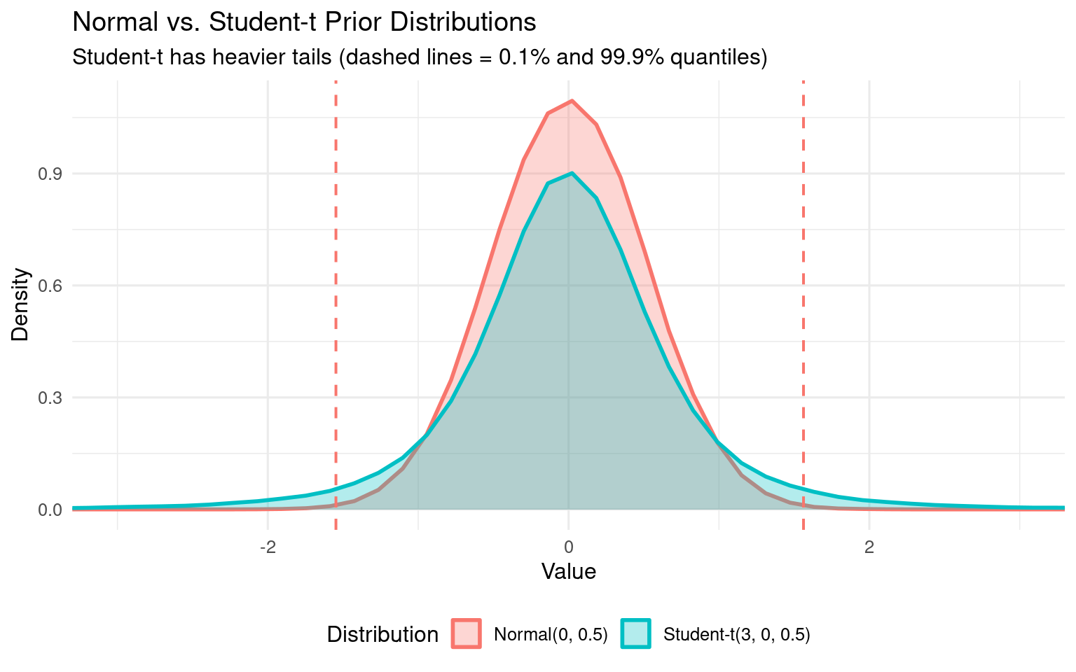
cat("Student-t allows extreme values 2x more likely than normal!\n\n")
Student-t allows extreme values 2x more likely than normal!
Show code
# Graphical comparison
library(ggplot2)
comparison_df <- data.frame(
  value = c(normal_samples, studentt_samples),
  distribution = rep(c("Normal(0, 0.5)", "Student-t(3, 0, 0.5)"), each = n_samples)
)

ggplot(comparison_df, aes(x = value, fill = distribution, color = distribution)) +
  geom_density(alpha = 0.3, linewidth = 1) +
  geom_vline(xintercept = normal_99, linetype = "dashed", color = "#F8766D", linewidth = 0.7) +
  geom_vline(xintercept = studentt_99, linetype = "dashed", color = "#00BFC4", linewidth = 0.7) +
  coord_cartesian(xlim = c(-3, 3)) +
  scale_fill_manual(values = c("#F8766D", "#00BFC4")) +
  scale_color_manual(values = c("#F8766D", "#00BFC4")) +
  labs(
    title = "Normal vs. Student-t Prior Distributions",
    subtitle = "Student-t has heavier tails (dashed lines = 0.1% and 99.9% quantiles)",
    x = "Value",
    y = "Density",
    fill = "Distribution",
    color = "Distribution"
  ) +
  theme_minimal(base_size = 12) +
  theme(legend.position = "bottom")

When to use each:

  • Student-t: Default choice (conservative, robust to outliers)
  • Normal: When you have strong domain knowledge about plausible ranges (better for RT data in controlled experiments)

Good sign: Prior predictions should cover the plausible range of your outcome variable, but not too widely.

1.4 Summary

Key takeaways:

  1. Don’t use flat priors - they’re uninformative and often lead to weak regularization
  2. Default intercept priors adapt to data - implicit assumptions depend on your coding!
  3. Specify priors explicitly based on domain knowledge
  4. Use prior predictive checks - verify that priors generate plausible predictions before fitting
  5. Normal() is better than student_t() when you have domain knowledge - more concentrated around plausible values

Next steps: - See 02_prior_predictive_checks_rt.qmd for detailed prior validation - See 03_posterior_predictive_checks_rt.qmd for checking if the fitted model makes sense