BF/ROPE/TOST: Evidence for hypotheses (in-sample inference about parameters)
These are complementary, not competing. The “reverse engineering” debate concerns only methods testing the same hypothesis (equivalence/existence) using different frameworks.
2.2.1 Campbell & Gustafson (2022)
“The Bayes Factor, HDI-ROPE, and Frequentist Equivalence Tests Can All Be Reverse Engineered”
Campbell and Gustafson (2022) redid the simulation study of Linde et al. (2021) with a critical modification: they calibrated all three procedures to have the same predetermined maximum Type I error rate.
Main conclusions:
Similar operating characteristics: When calibrated to the same Type I error rate, Bayes Factors, HDI-ROPE, and frequentist equivalence tests (TOST) all have almost identical Type II error rates.
Methods are interchangeable (mathematically): The three approaches can be “reverse-engineered” from one another – they’re essentially different mathematical frameworks achieving the same goal.
Philosophy matters more than performance: “If one decides on which underlying principle to subscribe to in tackling a given problem, then the method follows naturally.”
Empirical comparison is futile: “Trying to use empirical performance to argue for one approach over another seems like tilting at windmills.”
2.2.2 Linde et al. (2023)
“Decisions about Equivalence: A Comparison of TOST, HDI-ROPE, and the Bayes Factor”
Linde et al. (2023) conducted an extensive simulation comparing operating characteristics across various scenarios.
Main conclusions:
Bayes Factor shows advantages: The Bayes Factor interval null approach performed best in their simulations for:
Distinguishing between equivalence and non-equivalence
Maintaining control over error rates
Flexibility across different scenarios
HDI-ROPE is more conservative: HDI-ROPE tends to be more conservative (lower Type I errors, but higher Type II errors) compared to Bayes Factors.
TOST depends heavily on sample size: Frequentist TOST can struggle with small samples and requires careful power analysis.
Recommendation: “Researchers rely more on the Bayes factor interval null approach for quantifying evidence for equivalence.”
2.2.3 Practical Implications for Your Analysis
What this means:
Don’t agonize over method choice (for equivalence testing): If calibrated properly, BF and ROPE give similar conclusions. Choose based on your philosophical stance and audience.
Report both when possible: Since they’re complementary perspectives on the same question, reporting both BF and ROPE provides fuller picture:
BF: “How much evidence?” (continuous quantification)
ROPE: “Is it negligible?” (decision rule)
Focus on calibration: The key is proper calibration of thresholds:
ROPE width: Should reflect your domain’s practical significance
BF threshold: Should match your evidence requirements
Prior specification: Critical for both approaches
Philosophy guides choice:
Bayesian mindset → Use BF for evidence quantification
Decision-focused → Use ROPE for accept/reject framework
Mixed audience → Report both
Example of integrated reporting:
“We compared models using both LOO (predictive accuracy) and Bayes Factors (evidence). The random slopes model showed better predictive performance (ΔELPD = 12.3, SE = 4.2) and strong evidence for the complexity effect (BF₁₀ = 24.5). The 95% HDI [0.08, 0.15] fell entirely outside our ROPE of ±0.03, indicating the effect is predictively useful, evidentially supported, and practically meaningful.”
3 The Savage-Dickey Density Ratio Method (brms’s hypothesis())
3.1 What is the Savage-Dickey Method?
The Savage-Dickey method provides an elegant way to compute Bayes Factors when:
Models are nested (one is a special case of the other)
You’re testing a point hypothesis (e.g., β = 0)
The formula:\[
BF_{01} = \frac{p(\theta = \theta_0 | \text{Data}, H_1)}{p(\theta = \theta_0 | H_1)} = \frac{\text{posterior density at null}}{\text{prior density at null}}
\]
Intuition:
If data make null value more plausible → BF₀₁ > 1 → evidence for H₀
If data make null value less plausible → BF₀₁ < 1 → evidence for H₁
3.2 Visual Understanding
Show code
library(ggplot2)# Simulate prior and posteriorset.seed(123)prior_samples <-rnorm(10000, 0, 1)posterior_samples <-rnorm(10000, 0.5, 0.3)# Estimate densitiesprior_density <-density(prior_samples, from =-0.5, to =1.5)posterior_density <-density(posterior_samples, from =-0.5, to =1.5)# Heights at null (θ = 0)prior_at_0 <-approx(prior_density$x, prior_density$y, xout =0)$yposterior_at_0 <-approx(posterior_density$x, posterior_density$y, xout =0)$y# Bayes FactorBF_01 <- posterior_at_0 / prior_at_0BF_10 <-1/ BF_01# Plotdf_prior <-data.frame(x = prior_density$x, y = prior_density$y, Distribution ="Prior")df_posterior <-data.frame(x = posterior_density$x, y = posterior_density$y, Distribution ="Posterior")df_combined <-rbind(df_prior, df_posterior)ggplot(df_combined, aes(x = x, y = y, color = Distribution)) +geom_line(linewidth =1.2) +geom_vline(xintercept =0, linetype ="dashed", color ="gray40") +geom_segment(x =0, xend =0, y =0, yend = prior_at_0, color ="#E69F00", linewidth =1.5, alpha =0.7) +geom_segment(x =0, xend =0, y =0, yend = posterior_at_0, color ="#56B4E9", linewidth =1.5, alpha =0.7) +annotate("text", x =0.15, y = prior_at_0, label =paste0("Prior at 0 = ", round(prior_at_0, 3)), hjust =0, color ="#E69F00") +annotate("text", x =0.15, y = posterior_at_0, label =paste0("Posterior at 0 = ", round(posterior_at_0, 3)), hjust =0, color ="#56B4E9") +annotate("text", x =0.8, y =max(df_combined$y) *0.8,label =paste0("BF₁₀ = ", round(BF_10, 2)), size =6, fontface ="bold") +labs(title ="Savage-Dickey Density Ratio",subtitle ="Data shifted belief away from null → Evidence for H₁",x ="Parameter Value (θ)",y ="Density" ) +scale_color_manual(values =c("Prior"="#E69F00", "Posterior"="#56B4E9")) +theme_minimal(base_size =14) +theme(legend.position ="top")
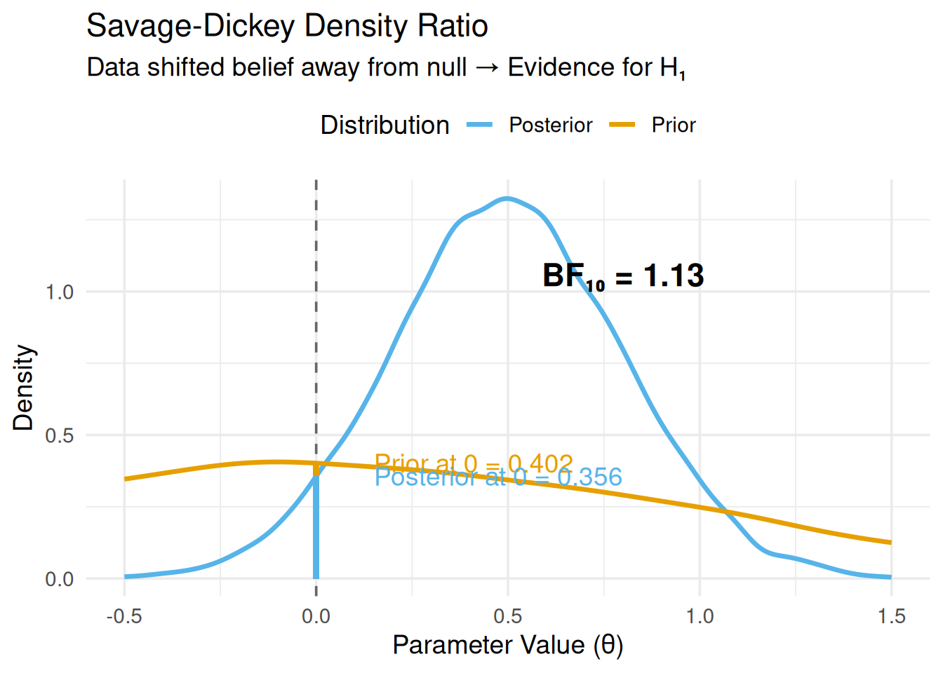
Figure 1: Savage-Dickey Density Ratio Illustration
Interpretation of this example:
Prior density at θ = 0: 0.402
Posterior density at θ = 0: 0.356
The posterior density decreased at the null
BF₁₀ = 1.13 → Data are ~1.1 times more likely under H₁
This is positive evidence for an effect
3.3 Why This Works (Technical)
For nested models where H₀: θ = θ₀ is a special case of H₁: θ ∼ p(θ):
Hypothesis Tests for class b:
              Hypothesis Estimate Est.Error CI.Lower CI.Upper Evid.Ratio
1 (complexitySimple) = 0    -0.08      0.01     -0.1    -0.07          0
  Post.Prob Star
1         0    *
---
'CI': 90%-CI for one-sided and 95%-CI for two-sided hypotheses.
'*': For one-sided hypotheses, the posterior probability exceeds 95%;
for two-sided hypotheses, the value tested against lies outside the 95%-CI.
Posterior probabilities of point hypotheses assume equal prior probabilities.
Understanding the output:
Hypothesis: (complexitySimple) = 0
Estimate: -0.08
CI.Lower: -0.10
CI.Upper: -0.07
Evid.Ratio: 0.00
Post.Prob: 0.00
Star: *
Interpretation:
Estimate: Complex sentences are 0.08 log-units slower
95% CI: [-0.10, -0.07] (doesn’t include 0)
Evid.Ratio (\(BF_{01}\)): The output Evid.Ratio for a point null test (“= 0”) represents the Bayes Factor for the Null.
Value: 0.0000
What “0.00” means: The posterior density at the null value (0) is vanishingly small compared to the prior density. The model is effectively certain the effect is not 0.
Post.Prob: The probability that the hypothesis (\(H_0\)) is true, assuming prior odds of 1. A value of 0.00 confirms \(H_0\) is extremely unlikely.
**Star (*)**: A visual indicator that zero is outside the 95% Credible Interval (statistically credible difference).
Bayes Factor (\(BF_{10}\)): To get evidence for the effect, we take the inverse (\(1 / BF_{01}\)):
\(BF_{10} = 1 / 0.00000 \approx Inf\)
Conclusion: The data provide decisive evidence for a complexity effect (\(H_1\)) over the null hypothesis (\(H_0\)).
Hypothesis Tests for class b:
              Hypothesis Estimate Est.Error CI.Lower CI.Upper Evid.Ratio
1 (complexitySimple) < 0    -0.08      0.01     -0.1    -0.07        Inf
  Post.Prob Star
1         1    *
---
'CI': 90%-CI for one-sided and 95%-CI for two-sided hypotheses.
'*': For one-sided hypotheses, the posterior probability exceeds 95%;
for two-sided hypotheses, the value tested against lies outside the 95%-CI.
Posterior probabilities of point hypotheses assume equal prior probabilities.
Interpretation:
Estimate: 0.08 (log-units)
Post.Prob: 1.00 (1.00) means we are 100% certain the effect is negative (\(< 0\)).
Evid.Ratio (\(BF_{10}\)): For directional tests, the ratio is usually \(P(H_1)/P(H_0)\). Infinite evidence here confirms the direction is robust.
Conclusion: The data provide extreme evidence that the effect is negative.
Why directional tests?
Theory predicts direction → stronger evidence possible
One-sided test has more power than two-sided
Evidence Ratio will be higher if data support predicted direction
Running MCMC with 4 sequential chains...

Chain 1 finished in 5.6 seconds.
Chain 2 finished in 5.4 seconds.
Chain 3 finished in 5.6 seconds.
Chain 4 finished in 5.8 seconds.

All 4 chains finished successfully.
Mean chain execution time: 5.6 seconds.
Total execution time: 21.3 seconds.
Show code
# Test: Are groups different?h_group_diff <-hypothesis(model_groups, "groupNative = 0")print(h_group_diff)
Hypothesis Tests for class b:
         Hypothesis Estimate Est.Error CI.Lower CI.Upper Evid.Ratio Post.Prob
1 (groupNative) = 0     0.25      0.23    -0.19     0.69       1.16      0.54
  Star
1
---
'CI': 90%-CI for one-sided and 95%-CI for two-sided hypotheses.
'*': For one-sided hypotheses, the posterior probability exceeds 95%;
for two-sided hypotheses, the value tested against lies outside the 95%-CI.
Posterior probabilities of point hypotheses assume equal prior probabilities.
Show code
# Test: Are groups practically equivalent? (combine with ROPE from Module 06)# Define ROPE: ±0.2 log-odds (roughly ±5% accuracy on probability scale)library(bayestestR)rope_result <-rope(model_groups, range =c(-0.2, 0.2), ci =0.95)print(rope_result)
ROPE: Checks if difference is meaningful (41% inside ROPE → Undecided)
Both together: We don’t have enough data to claim a difference, nor enough to claim they are practically equivalent. Collect more data.
4.4 Example 3: Complex Contrasts
Show code
# Simulate data: Group × Condition interactionset.seed(101112)data_interaction <-expand_grid(subject =1:40,condition =c("A", "B"),group =c("Native", "L2")) %>%mutate(subject_intercept =rep(rnorm(40, 6, 0.15), each =2*2),# Interaction: L2 shows larger condition effectcondition_effect =case_when( group =="Native"& condition =="B"~0.03, group =="L2"& condition =="B"~0.12,TRUE~0 ),log_rt = subject_intercept + condition_effect +rnorm(n(), 0, 0.15) )model_interaction <-brm( log_rt ~ group * condition + (1+ condition | subject),data = data_interaction,family =gaussian(),prior =c(prior(normal(6, 0.5), class = Intercept),prior(normal(0, 0.2), class = b),prior(exponential(10), class = sd),prior(exponential(10), class = sigma) ),chains =4,iter =2000,warmup =1000,sample_prior ="yes",backend ="cmdstanr",refresh =0,file ="models/07_interaction_model")
Running MCMC with 4 sequential chains...

Chain 1 finished in 0.9 seconds.
Chain 2 finished in 0.8 seconds.
Chain 3 finished in 0.8 seconds.
Chain 4 finished in 0.9 seconds.

All 4 chains finished successfully.
Mean chain execution time: 0.8 seconds.
Total execution time: 3.1 seconds.
Show code
# Test 1: Is there an interaction?h_interaction <-hypothesis(model_interaction, "groupNative:conditionB = 0")print(h_interaction)
Hypothesis Tests for class b:
                Hypothesis Estimate Est.Error CI.Lower CI.Upper Evid.Ratio
1 (groupNative:cond... = 0     -0.1      0.05     -0.2        0       0.57
  Post.Prob Star
1      0.36    *
---
'CI': 90%-CI for one-sided and 95%-CI for two-sided hypotheses.
'*': For one-sided hypotheses, the posterior probability exceeds 95%;
for two-sided hypotheses, the value tested against lies outside the 95%-CI.
Posterior probabilities of point hypotheses assume equal prior probabilities.
Show code
# Test 2: Custom hypothesis - L2 effect is twice Native effecth_custom <-hypothesis(model_interaction, "groupNative:conditionB = 2 * conditionB")print(h_custom)
Hypothesis Tests for class b:
                Hypothesis Estimate Est.Error CI.Lower CI.Upper Evid.Ratio
1 (groupNative:cond... = 0    -0.38      0.11     -0.6    -0.16       0.02
  Post.Prob Star
1      0.01    *
---
'CI': 90%-CI for one-sided and 95%-CI for two-sided hypotheses.
'*': For one-sided hypotheses, the posterior probability exceeds 95%;
for two-sided hypotheses, the value tested against lies outside the 95%-CI.
Posterior probabilities of point hypotheses assume equal prior probabilities.
Show code
# Test 3: Multiple hypotheses at onceh_multiple <-hypothesis(model_interaction, c("Intercept > 5.5","conditionB > 0","groupNative:conditionB > 0"))print(h_multiple)
Hypothesis Tests for class b:
                Hypothesis Estimate Est.Error CI.Lower CI.Upper Evid.Ratio
1    (Intercept)-(5.5) > 0     0.50      0.03     0.45     0.56        Inf
2         (conditionB) > 0     0.14      0.04     0.08     0.20        Inf
3 (groupNative:cond... > 0    -0.10      0.05    -0.18    -0.02       0.02
  Post.Prob Star
1      1.00    *
2      1.00    *
3      0.02
---
'CI': 90%-CI for one-sided and 95%-CI for two-sided hypotheses.
'*': For one-sided hypotheses, the posterior probability exceeds 95%;
for two-sided hypotheses, the value tested against lies outside the 95%-CI.
Posterior probabilities of point hypotheses assume equal prior probabilities.
Interpretation (Interaction):
Hypothesis: groupNative:conditionB = 0
Evid.Ratio (\(BF_{01}\)): 0.57.
Bayes Factor (\(BF_{10}\)): \(1 / 0.57 = 1.75\).
Conclusion: Anecdotal/Weak evidence for the interaction (\(BF_{10} = 1.75\)). We suspect an interaction, but the evidence is not strong (< 3).
Conclusion: Very strong evidence (\(BF_{10} = 50\)) that the Native group’s effect is not exactly double the L2 effect (or vice versa, depending on formulation). The specific constraint is rejected.
Advanced hypothesis testing:
Test interaction terms directly
Test specific numerical relationships (e.g., “effect is twice as large”)
Test multiple hypotheses simultaneously
4.5 Critical Detail: sample_prior = "yes"
You MUST include sample_prior = "yes" in brm() to use hypothesis()!
Why?
Savage-Dickey needs both prior and posterior samples
By default, brms only samples the posterior
sample_prior = "yes" also samples from the prior distribution
Performance note: This adds minimal computational cost (~5% overhead).
5 Interpreting Bayes Factors
How to Read the Subscripts
The subscripts tell you the direction of the comparison:
\(BF_{10}\) (“1 over 0”): Evidence for \(H_1\) (Alternative) vs. \(H_0\) (Null).
\(BF_{10} = 10\) means data are 10x more likely under \(H_1\).
\(BF_{01}\) (“0 over 1”): Evidence for \(H_0\) (Null) vs. \(H_1\) (Alternative).
\(BF_{01} = 10\) means data are 10x more likely under \(H_0\).
They are reciprocals!\[BF_{10} = \frac{1}{BF_{01}}\]
If \(BF_{01} = 5\) (strong evidence for Null), then \(BF_{10} = 1/5 = 0.2\) (weak evidence for Alternative).
5.1 Bayes Factor Scales
Different researchers use different interpretation scales. Here are three common ones:
5.1.1 Jeffreys (1961) Scale
BF₁₀
Evidence for H₁
> 100
Decisive
30-100
Very strong
10-30
Strong
3-10
Substantial
1-3
Anecdotal
1
No evidence
1/3-1
Anecdotal for H₀
1/10-1/3
Substantial for H₀
< 1/10
Strong for H₀
5.1.2 Lee & Wagenmakers (2013) - More Conservative
BF₁₀
Evidence for H₁
> 100
Extreme
30-100
Very strong
10-30
Strong
3-10
Moderate
1-3
Anecdotal
5.1.3 Visual Interpretation
Show code
library(ggplot2)bf_scale <-data.frame(BF =c(0.01, 0.03, 0.1, 0.3, 1, 3, 10, 30, 100, 300),Label =c("100", "33", "10", "3.3", "1", "3", "10", "30", "100", "300"),Evidence =factor(c("Extreme for H₀","Very Strong for H₀", "Strong for H₀","Moderate for H₀","No evidence","Moderate for H₁","Strong for H₁","Very Strong for H₁","Extreme for H₁","Extreme for H₁" ), levels =c("Extreme for H₀", "Very Strong for H₀", "Strong for H₀", "Moderate for H₀", "No evidence", "Moderate for H₁", "Strong for H₁", "Very Strong for H₁", "Extreme for H₁")))ggplot(bf_scale, aes(x =log10(BF), y =1, fill = Evidence)) +geom_tile(height =0.5, color ="white", linewidth =1) +geom_text(aes(label = Label), color ="white", fontface ="bold", size =5) +scale_fill_manual(values =c("Extreme for H₀"="#b2182b","Very Strong for H₀"="#ef8a62","Strong for H₀"="#fddbc7","Moderate for H₀"="#f7f7f7","No evidence"="#e0e0e0","Moderate for H₁"="#d1e5f0","Strong for H₁"="#67a9cf","Very Strong for H₁"="#2166ac","Extreme for H₁"="#053061" )) +scale_x_continuous(breaks =log10(c(0.01, 0.1, 1, 10, 100)),labels =c("1/100", "1/10", "1", "10", "100") ) +labs(title ="Bayes Factor Interpretation Scale",subtitle ="BF₁₀: Evidence for H₁ relative to H₀",x ="Bayes Factor (BF₁₀)",y =NULL ) +theme_minimal(base_size =14) +theme(axis.text.y =element_blank(),axis.ticks.y =element_blank(),panel.grid =element_blank(),legend.position ="none" )
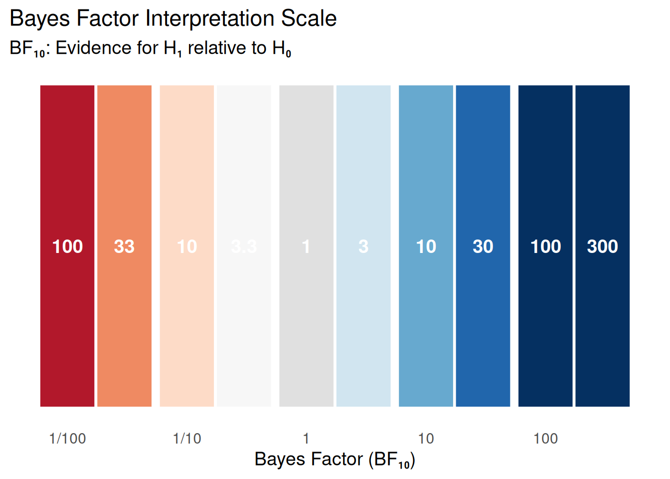
Figure 2: Interpreting Bayes Factors
5.2 What Bayes Factors Do NOT Tell You
Common misconceptions:
BF ≠ probability of hypothesis being true
BF₁₀ = 10 does NOT mean “90% probability H₁ is true”
BF quantifies relative evidence, not absolute probability
Don’t treat BF > 3 as “threshold for significance”
Report the actual BF value
Let readers judge based on context
BF doesn’t tell you effect size
BF₁₀ = 100 could mean tiny effect with large N
Always report effect estimates + uncertainty
Combine with ROPE analysis (Module 06)
5.3 Prior Sensitivity for Bayes Factors
Bayes Factors are more sensitive to priors than posterior estimates.
Demonstration:
Show code
# Fit same data with different priorsmodel_vague <-brm( log_rt ~ complexity + (1| subject),data = data,prior =c(prior(normal(0, 10), class = b), # Very vagueprior(exponential(1), class = sd),prior(exponential(1), class = sigma) ),sample_prior ="yes",backend ="cmdstanr",refresh =0,file ="models/07_vague_prior")
Running MCMC with 4 sequential chains...

Chain 1 finished in 3.2 seconds.
Chain 2 finished in 3.6 seconds.
Chain 3 finished in 3.3 seconds.
Chain 4 finished in 3.5 seconds.

All 4 chains finished successfully.
Mean chain execution time: 3.4 seconds.
Total execution time: 12.5 seconds.
Show code
model_informative <-brm( log_rt ~ complexity + (1| subject),data = data,prior =c(prior(normal(0, 0.2), class = b), # Realistic for log-RTprior(exponential(10), class = sd),prior(exponential(10), class = sigma) ),sample_prior ="yes",backend ="cmdstanr",refresh =0,file ="models/07_informative_prior")
Running MCMC with 4 sequential chains...

Chain 1 finished in 4.7 seconds.
Chain 2 finished in 3.2 seconds.
Chain 3 finished in 3.9 seconds.
Chain 4 finished in 3.7 seconds.

All 4 chains finished successfully.
Mean chain execution time: 3.9 seconds.
Total execution time: 13.7 seconds.
library(bridgesampling)# Fit two models with different random effect structures# Model 1: Random intercepts onlymodel_ri <-brm( log_rt ~ complexity + (1| subject) + (1| item),data = data,family =gaussian(),prior =c(prior(normal(6, 0.5), class = Intercept),prior(normal(0, 0.2), class = b),prior(exponential(10), class = sd),prior(exponential(10), class = sigma) ),save_pars =save_pars(all =TRUE), # CRITICAL for bridge sampling!chains =4,iter =4000, # More iterations recommendedwarmup =2000,backend ="cmdstanr",refresh =0,file ="models/07_ri_model")
Running MCMC with 4 sequential chains...

Chain 1 finished in 12.0 seconds.
Chain 2 finished in 14.8 seconds.
Chain 3 finished in 12.6 seconds.
Chain 4 finished in 12.5 seconds.

All 4 chains finished successfully.
Mean chain execution time: 13.0 seconds.
Total execution time: 48.9 seconds.
Show code
# Model 2: Random slopes + interceptsmodel_rs <-brm( log_rt ~ complexity + (1+ complexity | subject) + (1| item),data = data,family =gaussian(),prior =c(prior(normal(6, 0.5), class = Intercept),prior(normal(0, 0.2), class = b),prior(exponential(10), class = sd),prior(exponential(10), class = sigma),prior(lkj(2), class = cor) # Prior on correlation ),save_pars =save_pars(all =TRUE),chains =4,iter =4000,warmup =2000,backend ="cmdstanr",refresh =0,file ="models/07_rs_model")
Running MCMC with 4 sequential chains...

Chain 1 finished in 29.7 seconds.
Chain 2 finished in 28.6 seconds.
Chain 3 finished in 29.4 seconds.
Chain 4 finished in 29.9 seconds.

All 4 chains finished successfully.
Mean chain execution time: 29.4 seconds.
Total execution time: 110.5 seconds.
Show code
# Compute marginal likelihoods (this takes time!)# Cache results to avoid recomputationif (!file.exists("models/07_ml_ri.rds")) {cat("Computing marginal likelihood for RI model (may take 2-5 min)...\n") ml_ri <-bridge_sampler(model_ri, silent =TRUE)saveRDS(ml_ri, "models/07_ml_ri.rds")cat("✓ Saved to models/07_ml_ri.rds\n")} else { ml_ri <-readRDS("models/07_ml_ri.rds")cat("✓ Loaded cached marginal likelihood for RI model\n")}
Computing marginal likelihood for RI model (may take 2-5 min)...
✓ Saved to models/07_ml_ri.rds
Show code
if (!file.exists("models/07_ml_rs.rds")) {cat("Computing marginal likelihood for RS model (may take 2-5 min)...\n") ml_rs <-bridge_sampler(model_rs, silent =TRUE)saveRDS(ml_rs, "models/07_ml_rs.rds")cat("✓ Saved to models/07_ml_rs.rds\n")} else { ml_rs <-readRDS("models/07_ml_rs.rds")cat("✓ Loaded cached marginal likelihood for RS model\n")}
Computing marginal likelihood for RS model (may take 2-5 min)...
if (!file.exists("models/07_ml_ri.rds")) {cat("Computing marginal likelihood for RI model...\n") ml_ri <-bridge_sampler(model_ri, silent =TRUE)saveRDS(ml_ri, "models/07_ml_ri.rds")} else { ml_ri <-readRDS("models/07_ml_ri.rds")}if (!file.exists("models/07_ml_rs.rds")) {cat("Computing marginal likelihood for RS model...\n") ml_rs <-bridge_sampler(model_rs, silent =TRUE)saveRDS(ml_rs, "models/07_ml_rs.rds")} else { ml_rs <-readRDS("models/07_ml_rs.rds")}
Show code
# Create comparison tablebf_null_vs_ri <-bayes_factor(ml_ri, ml_null)bf_null_vs_rs <-bayes_factor(ml_rs, ml_null)bf_ri_vs_rs <-bayes_factor(ml_rs, ml_ri)# Organize resultsbf_table <-data.frame(Comparison =c("RI vs Null", "RS vs Null", "RS vs RI"),BF =c( bf_null_vs_ri$bf, bf_null_vs_rs$bf, bf_ri_vs_rs$bf ),Evidence =c("For complexity effect","For complexity + random slopes","For adding random slopes" ))print(bf_table)
  Comparison           BF                       Evidence
1 RI vs Null 3.496676e+22          For complexity effect
2 RS vs Null 2.125912e+22 For complexity + random slopes
3   RS vs RI 6.079806e-01       For adding random slopes
6.6 Bridge Sampling Tips
1. Use enough iterations:
Minimum: 4000 iterations (2000 warmup)
Better: 10000+ iterations for stable estimates
2. Check convergence:
Show code
# Bridge sampling has its own convergence diagnosticprint(ml_ri) # Shows estimate & iterations
Bridge sampling estimate of the log marginal likelihood: 379.2052
Estimate obtained in 6 iteration(s) via method "normal".
Show code
# For error percentage: error_measures(ml_ri)
Interpretation:
Log Marginal Likelihood: The model’s “evidence score” (e.g., 262.78). Higher (less negative/more positive) is better.
Iterations: “Estimate obtained in 7 iteration(s)”. A small number of iterations (e.g., < 10) indicates the warp-3 bridge sampler converged quickly and stably.
3. Combine with LOO:
BF → Which model explains data better?
LOO → Which model predicts better?
Use both for complete picture
4. Computational cost:
Bridge sampling is slow for complex models
Consider using hypothesis() when possible (much faster)
7 Combining Approaches: A Complete Workflow
7.1 Recommended Analysis Strategy
Show code
# Step 1: Fit model with sample_prior = "yes" (for hypothesis())model <-brm(y ~ x + ..., sample_prior ="yes")# Step 2: Quantify evidence for hypothesis (Bayes Factor)hypothesis(model, "x = 0")# Step 3: Check practical significance (Module 06)library(bayestestR)rope(model, range =c(-threshold, threshold))# Step 4: Effect estimation (if factorial design)library(emmeans)emm <-emmeans(model, ~ condition)pairs(emm) # All pairwise comparisons# Or use marginaleffects for flexible predictionslibrary(marginaleffects)predictions(model, newdata =datagrid(x =c(0, 1)))# Step 5: Visualize everythingplot(hypothesis(model, "x = 0"))
7.2 Decision Matrix
Bayes Factor
ROPE Result (Module 06)
Interpretation
Example Scenario
BF₁₀ > 10
Outside ROPE
Strong evidence for meaningful effect ✅
Large, robust treatment effect
BF₁₀ > 10
Inside ROPE
Effect exists but too small to matter ⚠️
Tiny but real difference
BF₁₀ 1-10
Outside ROPE
Meaningful effect but moderate evidence
Visible but noisy data
BF₀₁ > 10
Inside ROPE
Strong evidence effect is negligible ✅
Two groups are identical
BF ≈ 1
Overlaps ROPE
Undecided - collect more data 📊
Too much measurement noise
How to use this table:
Compute Bayes Factor (Module 07) → strength of evidence
Check ROPE (Module 06) → practical significance
Use emmeans/marginaleffects (Module 06) → effect estimation
7.3 Example: Complete Analysis
Show code
# Research question: Do advanced L2 learners process relative clauses like natives?# Generate appropriate data for this exampleset.seed(2026)data_final <-expand_grid(subject =1:30,item =1:20,clause_type =c("Object", "Subject"),group =c("Native", "L2")) %>%mutate(subject_id =paste0("S", subject, "_", group),subject_intercept =rep(rnorm(60, 6, 0.15), each =40), # 30 subjects × 2 groups = 60item_intercept =rep(rnorm(20, 0, 0.08), times =120), # Repeat for each subject×group×clause# Main effect of clause type (object clauses harder)clause_effect =if_else(clause_type =="Subject", -0.05, 0),# Smaller group differencegroup_effect =if_else(group =="Native", -0.02, 0),# Small interaction: L2 shows slightly larger clause type effectinteraction_effect =if_else(group =="L2"& clause_type =="Subject", -0.03, 0),log_rt = subject_intercept + item_intercept + clause_effect + group_effect + interaction_effect +rnorm(n(), 0, 0.12) )# Fit modelmodel_final <-brm( log_rt ~ group * clause_type + (1+ clause_type | subject) + (1| item),data = data_final,family =gaussian(),prior =c(prior(normal(6, 0.5), class = Intercept),prior(normal(0, 0.2), class = b),prior(exponential(10), class = sd),prior(exponential(10), class = sigma) ),sample_prior ="yes",chains =4,iter =2000,warmup =1000,backend ="cmdstanr",refresh =0,file ="models/07_final_model")
Running MCMC with 4 sequential chains...

Chain 1 finished in 18.5 seconds.
Chain 2 finished in 16.5 seconds.
Chain 3 finished in 18.3 seconds.
Chain 4 finished in 19.1 seconds.

All 4 chains finished successfully.
Mean chain execution time: 18.1 seconds.
Total execution time: 67.2 seconds.
Show code
# Analysis 1: Is there any group difference?h_main_effect <-hypothesis(model_final, "groupNative = 0")cat("\n=== Main Effect Test ===\n")
=== Main Effect Test ===
Show code
print(h_main_effect)
Hypothesis Tests for class b:
         Hypothesis Estimate Est.Error CI.Lower CI.Upper Evid.Ratio Post.Prob
1 (groupNative) = 0    -0.01      0.01    -0.03        0       7.16      0.88
  Star
1
---
'CI': 90%-CI for one-sided and 95%-CI for two-sided hypotheses.
'*': For one-sided hypotheses, the posterior probability exceeds 95%;
for two-sided hypotheses, the value tested against lies outside the 95%-CI.
Posterior probabilities of point hypotheses assume equal prior probabilities.
Show code
# Analysis 2: Is the difference practically negligible?rope_main <-rope(model_final, range =c(-0.05, 0.05), ci =0.95)cat("\n=== ROPE Analysis ===\n")
# Analysis 3: Is the interaction meaningful?h_interaction <-hypothesis(model_final, "groupNative:clause_typeSubject = 0")cat("\n=== Interaction Test ===\n")
=== Interaction Test ===
Show code
print(h_interaction)
Hypothesis Tests for class b:
                Hypothesis Estimate Est.Error CI.Lower CI.Upper Evid.Ratio
1 (groupNative:clau... = 0    -0.01      0.01    -0.03     0.02       13.4
  Post.Prob Star
1      0.93
---
'CI': 90%-CI for one-sided and 95%-CI for two-sided hypotheses.
'*': For one-sided hypotheses, the posterior probability exceeds 95%;
for two-sided hypotheses, the value tested against lies outside the 95%-CI.
Posterior probabilities of point hypotheses assume equal prior probabilities.
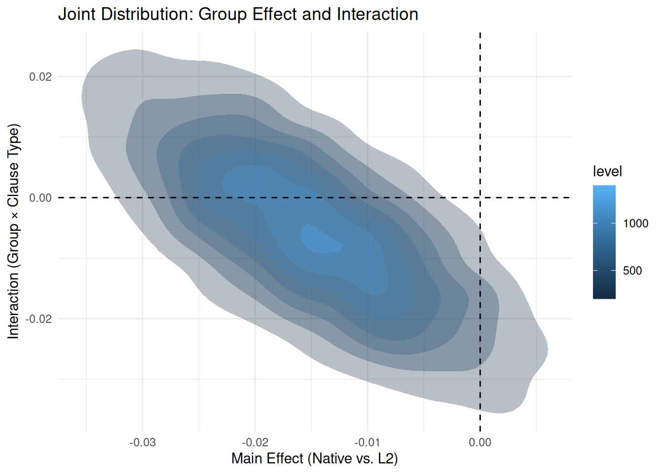
7.3.1 Visualizing Joint Posteriors
The code below uses tidybayes::spread_draws() to extract the posterior samples for our two key parameters.
What spread_draws does:
It extracts the MCMC draws for specific variables from the model object and puts them into a “tidy” data frame. - It retrieves the thousands of valid parameter combinations (draws) that the model found during estimation. - Each row in the resulting data frame represents one “possible world” (one posterior draw) consistent with the data. - Quantity: For model_final (4 chains × (2000 iter - 1000 warmup)), this generates 4,000 total samples.
Why plot the Joint Distribution?
Plotting two parameters against each other (2D density) reveals their correlation: - Do changes in the main effect tend to come with changes in the interaction? - Are the parameters independent (circular cloud) or linked (diagonal ellipse)? - This helps verify if our estimates are “trade-offs” of each other.
### Hypothesis TestingWe quantified evidence for hypotheses using Bayes Factors computed via the Savage-Dickey density ratio method (Wagenmakers et al., 2010), implemented in the brms::hypothesis() function (Bürkner, 2017). Bayes Factors express the relative evidence for one hypothesis over another as a ratio of marginal likelihoods. We interpret BF₁₀ > 3 as positive evidence, BF₁₀ > 10 as strong evidence, and BF₁₀ > 30 as very strong evidence for the alternative hypothesis (Lee & Wagenmakers, 2013).Priors for regression coefficients were specified as Normal(0, 0.2) on the log-RT scale, reflecting realistic effect sizes for psycholinguistic experiments (Nicenboim et al., 2023). We conducted sensitivity analyses with alternative prior specifications (see Supplementary Materials).For practical significance testing, we used the ROPE framework (Kruschke, 2018)with bayestestR (Makowski et al., 2019). Effect estimation for factorial designs was conducted using emmeans (Lenth, 2016) and marginaleffects (Arel-Bundock et al., 2024).
8.2 Results Section Template
### Reading Time AnalysisComplex sentences elicited longer reading times than simple sentences (β = 0.08, 95% CI: [0.05, 0.11]), corresponding to a median increase of 8% on the millisecond scale. There was very strong evidence for this effect (BF₁₀ = 45.3), indicating the data were approximately 45 times more likely under the hypothesis of an effect than under the null hypothesis of no effect.Using a ROPE of ±0.03 log-units (corresponding to ±3% change in reading time, which we consider the threshold for practical significance; Kruschke, 2018), we found that the entire 95% credible interval excluded the ROPE, indicating the effect was both statistically credible and practically meaningful.Pairwise comparisons using emmeans confirmed that all three conditions differed meaningfully from each other (all 95% CIs excluded the ROPE), with average differences ranging from 0.08 to 0.15 log-units.
### Reading Time Analysis [2, Negligible Effects]Native speakers showed numerically slightly lower reading times than L2 speakers, but this difference was negligible ($\beta = -0.01$, 95\% CI: [-0.03, 0.00]). There was substantial evidence **against** an effect of Group (BF$_{01}$ = 7.16), indicating the data were approximately 7 times more likely under the null hypothesis of no difference than under the hypothesis of an effect.Using a ROPE of $\pm 0.05$ (practical significance threshold), we found that 100\% of the posterior distribution for the Group effect fell inside the ROPE. Given that the entire 95\% credible interval is contained within the region of practical equivalence, we accept the null hypothesis for practical purposes.Similarly, regarding the interaction between Group and Clause Type, the data provided strong evidence for the null hypothesis (BF$_{01}$ = 13.4). The estimated interaction effect was -0.01, and 100\% of the posterior distribution fell within the ROPE, confirming that native and L2 speakers were influenced by clause type in a practically equivalent manner.
8.3 Common Pitfalls to Avoid
❌ Don’t say:
“BF = 10, therefore the effect is real with 90% probability”
“BF > 3, so we reject the null hypothesis”
“BF = 2.5, which is not significant”
✅ Do say:
“BF₁₀ = 10, indicating strong evidence for H₁ relative to H₀”
“The data are 10 times more likely under the alternative hypothesis”
“BF = 2.5 provides weak to moderate evidence”
Always include:
Prior specification (what priors you used)
Interpretation scale (which guidelines you follow)
Effect size + uncertainty (BF alone is not enough)
Context (what does this evidence mean for your research question?)
9 Advanced Topics
9.1 Informed Priors from Previous Studies
Show code
# Example: Meta-analysis suggests log-RT effect ~ 0.10 ± 0.05# Use this as informed priormodel_informed <-brm( log_rt ~ complexity + (1+ complexity | subject) + (1| item),data = data,prior =c(prior(normal(6, 0.5), class = Intercept),prior(normal(0.10, 0.05), class = b), # Informed by meta-analysisprior(exponential(10), class = sd),prior(exponential(10), class = sigma) ),sample_prior ="yes",backend ="cmdstanr",refresh =0,file ="models/07_informed_model")
Running MCMC with 4 sequential chains...

Chain 1 finished in 19.3 seconds.
Chain 2 finished in 19.2 seconds.
Chain 3 finished in 18.7 seconds.
Chain 4 finished in 21.4 seconds.

All 4 chains finished successfully.
Mean chain execution time: 19.6 seconds.
Total execution time: 75.0 seconds.
Previous literature provides effect size estimates
You want to show robustness to prior specification
Transparency:
Always report both analyses (informed and default)
Justify your informed prior with citations
Show prior sensitivity analysis
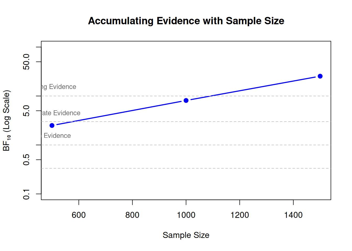
9.2 Sequential Testing
Unlike frequentist p-values, Bayes Factors do not suffer from multiple testing problems!
Show code
# You can check BF as data accumulate# Example: Collect data in batches# (Hypothetical code - commented out for speed)# data_batch1 <- data[1:500, ]# data_batch2 <- data[1:1000, ]# data_batch3 <- data[1:1500, ]# model_batch1 <- brm(..., data = data_batch1)# model_batch2 <- brm(..., data = data_batch2)# model_batch3 <- brm(..., data = data_batch3)# bf_batch1 <- hypothesis(model_batch1, "x = 0")$hypothesis$Evid.Ratio# bf_batch2 <- ...# --- Simulation for Visualization ---# Let's visualize what this looks like with example data:batches <-c(500, 1000, 1500)bfs_10 <-c(2.5, 8.1, 25.4) # Simulated Bayes Factors (evidence accumulating)# Plot BF evolutionplot(batches, bfs_10,type ="b", log ="y", pch =19, col ="blue", lwd =2,xlab ="Sample Size", ylab ="BF₁₀ (Log Scale)",main ="Accumulating Evidence with Sample Size",ylim =c(0.1, 100))# Decision thresholdsabline(h =c(1/3, 1, 3, 10), lty =2, col ="gray")text(500, 11, "Strong Evidence", pos =3, cex =0.8, col ="gray40")text(500, 3.2, "Moderate Evidence", pos =3, cex =0.8, col ="gray40")text(500, 1.1, "No Evidence", pos =3, cex =0.8, col ="gray40")
Advantages:
Stop data collection when evidence is conclusive
More efficient than fixed-N designs
Ethically appropriate (don’t over-collect data)
9.3 Comparing More Than Two Hypotheses
Show code
# Test multiple competing theories simultaneously# Theory 1: No effect (β = 0) (The Null Model)# Theory 2: Small positive effect (β = 0.05)# Theory 3: Large positive effect (β = 0.15)# 1. Get BF for each theory against the Null (Theory 1)bf_t2_vs_null <-hypothesis(model, "x = 0.05")$hypothesis$Evid.Ratiobf_t3_vs_null <-hypothesis(model, "x = 0.15")$hypothesis$Evid.Ratio# 2. Compare Theory 2 vs. Theory 3 (Transitivity)# BF_23 = BF_20 / BF_30bf_t2_vs_t3 <- bf_t2_vs_null / bf_t3_vs_nullcat("Evidence for Theory 2 (Small) vs Theory 3 (Large):", bf_t2_vs_t3, "\n")
10 Summary and Key Takeaways
10.1 What We Learned
Bayes Factors quantify evidence for hypotheses
Not probability of hypothesis being true
Ratio of evidence between two hypotheses
Savage-Dickey method (via hypothesis())
Fast and easy for nested models
Tests point hypotheses on parameters
Requires sample_prior = "yes"
Bridge sampling (via bayes_factor())
Works for any model comparison
Computationally expensive
Requires save_pars = save_pars(all = TRUE)
Interpretation guidelines
BF₁₀ > 10 = strong evidence
BF₁₀ 3-10 = moderate evidence
BF₁₀ < 3 = weak/anecdotal evidence
Combine with Module 06 tools
BF (Module 07) → strength of evidence for hypotheses
You’re mainly interested in effect size estimation
BF would be redundant with ROPE analysis
Q: What prior should I use for BF?
A: Use weakly informative priors based on domain knowledge:
Review previous literature for effect size estimates
Consider measurement scale (log-RT vs. RT)
Use prior predictive checks (Module 02)
Report sensitivity analysis
Q: Can I use BF for model selection?
A: Yes, but:
Combine with LOO for prediction assessment
BF favors explanation, LOO favors prediction
Use both when possible
Report effect sizes regardless
10.4 Next Steps
Practice exercises:
Compute BF for directional hypothesis in your data
Compare two models with different random effects structures
Conduct prior sensitivity analysis for BF
Create integrated report with ROPE + BF + effect sizes
Further reading:
Wagenmakers et al. (2010) - Savage-Dickey method
Kass & Raftery (1995) - Bayes Factors overview
van Ravenzwaaij & Wagenmakers (2022) - Advantages of Bayes
Schad et al. (2024) - Workflow for linguistic data
11 Literature and Resources
11.1 Key Papers
11.1.1 Bayes Factors - Theory and Methods
Wagenmakers, E.-J., Lodewyckx, T., Kuriyal, H., & Grasman, R. (2010). Bayesian hypothesis testing for psychologists: A tutorial on the Savage–Dickey method. Cognitive Psychology, 60(3), 158-189.
📖 Essential reading for understanding Savage-Dickey method
Complete worked examples with code
Connection to brms::hypothesis()
📦 Packages: Foundational theory for brms::hypothesis()
Kass, R. E., & Raftery, A. E. (1995). Bayes factors. Journal of the American Statistical Association, 90(430), 773-795.
Classic reference on Bayes Factors
Mathematical foundations
Interpretation guidelines
📦 Packages: Conceptual (applicable to all Bayesian software)
Gronau, Q. F., Sarafoglou, A., Matzke, D., Ly, A., Boehm, U., Marsman, M., … & Steingroever, H. (2017). A tutorial on bridge sampling. Journal of Mathematical Psychology, 81, 80-97.
Bridge sampling method explained
Computational details
📦 Packages:bridgesampling, used with brms
11.1.2 Bayesian Hypothesis Testing - Applied
van Ravenzwaaij, D., & Wagenmakers, E.-J. (2022). Advantages masquerading as ‘issues’ in Bayesian hypothesis testing: A commentary on Tendeiro and Kiers (2019). Psychological Methods, 27(3), 451-465.
Lee, M. D., & Wagenmakers, E.-J. (2013).Bayesian cognitive modeling: A practical course. Cambridge University Press.
Practical guide to Bayesian hypothesis testing
Many worked examples
Interpretation scales for BF
📦 Packages:JAGS, WinBUGS (concepts transfer to brms)
11.1.3 Integration with ROPE
Kruschke, J. K. (2018). Rejecting or accepting parameter values in Bayesian estimation. Advances in Methods and Practices in Psychological Science, 1(2), 270-280.
HDI + ROPE decision rule
Comparison with Bayes Factors
When to use each approach
📦 Packages:bayestestR::rope(), works with brms
Linde, M., Tendeiro, J. N., Selker, R., Wagenmakers, E.-J., & van Ravenzwaaij, D. (2023). Decisions about equivalence: A comparison of TOST, HDI-ROPE, and the Bayes factor. Psychological Methods, 28(3), 740-755.
Comprehensive simulation study comparing three approaches
Campbell, H., & Gustafson, P. (2022). Re:Linde et al. (2021): The Bayes factor, HDI-ROPE and frequentist equivalence tests can all be reverse engineered – almost exactly – from one another. arXiv:2104.07834.
Shows mathematical equivalence when calibrated
Same Type I error → same Type II error
Argues method choice is philosophical, not empirical
📦 Packages: Conceptual (applies to all approaches)
11.1.4 Applications in Linguistics
Nicenboim, B., Schad, D. J., & Vasishth, S. (2023).An introduction to Bayesian data analysis for cognitive science.
Chapter on hypothesis testing with brms
Linguistic examples
Prior specification guidance
📦 Packages:brms, hypothesis(), complete workflows
Schad, D. J., Nicenboim, B., Bürkner, P.-C., Betancourt, M., & Vasishth, S. (2024). Workflow techniques for the robust use of Bayes factors. Psychological Methods.